© 2015 McGraw-Hill Education. All rights reserved. Chapter 18 Inventory Theory.
37
© 2015 McGraw-Hill Education. All rights reserved. © 2015 McGraw-Hill Education. All rights reserved. Frederick S. Hillier Gerald J. Lieberman Chapter 18 Inventory Theory
-
Upload
robert-white -
Category
Documents
-
view
214 -
download
0
Transcript of © 2015 McGraw-Hill Education. All rights reserved. Chapter 18 Inventory Theory.
© 2015 McGraw-Hill Education. All rights reserved.
© 2015 McGraw-Hill Education. All rights reserved.
Frederick S. Hillier Gerald J. Lieberman
Chapter 18
Inventory Theory

© 2015 McGraw-Hill Education. All rights reserved.
Introduction
• Scientific inventory management– Mathematical model describes system
behavior
– Goal: optimal inventory policy with respect to the model
– Computerized information processing system maintains inventory level records
– Apply the inventory policy to replenish inventory
2
© 2015 McGraw-Hill Education. All rights reserved.
Introduction
• Demand– Number of units that will need to be withdrawn
from inventory
• Deterministic inventory model– Used when demand is known
• Stochastic inventory model– Used when demand cannot be predicted well
3

© 2015 McGraw-Hill Education. All rights reserved.
18.1 Examples
• Example 1: manufacturing speakers for TV sets– One speaker needed per TV set
• Sets manufactured on continuous production line
– Speakers produced in batches• $12,000 setup cost per batch
– $10 unit production cost of a single speaker
– $0.30 per month holding cost per speaker
– $1.10 per month shortage cost
4

© 2015 McGraw-Hill Education. All rights reserved.
Examples
• Example 2: wholesale bicycle distribution– Distributor purchases a specific bicycle model
from the manufacturer and supplies it to various bike shops
– Demand is uncertain
– Ordering cost includes administrative cost of $2000 and unit cost of $350 per bicycle
– $10 per bicycle holding cost
– $150 per bicycle shortage cost
5

© 2015 McGraw-Hill Education. All rights reserved.
6
• Cost of ordering z units– Includes a static cost and a cost per unit
• K is the setup cost and c is the unit cost
• Holding cost– Represents all costs associated with holding a
unit in inventory until it is sold or used• Cost of tied-up capital
• Space
• Insurance
• Protection
18.2 Components of Inventory Models

© 2015 McGraw-Hill Education. All rights reserved.
7
• Shortage cost– Also called unsatisfied demand cost
– Cost incurred when demand exceeds available stock
• Backlogging: demand not lost but delayed
• No backlogging: orders are canceled or met by priority shipment
– Revenue may or may not be included in the model
Components of Inventory Models
© 2015 McGraw-Hill Education. All rights reserved.
8
• Salvage cost– Negative of the salvage value
– Included in the holding cost
• Discount rate– Accounts for the time value of money
• Classification of inventory model based on how often inventory is monitored– Continuous review
– Periodic review
Components of Inventory Models
© 2015 McGraw-Hill Education. All rights reserved.
18.3 Deterministic Continuous-Review Models
• Economic order quantity (EOQ) model – Stock levels are depleted over time
• Replenished by a batch shipment
• Basic EOQ model assumptions– Demand rate is constant at d units per unit
time
– Order quantity Q to replenish inventory levels arrives all at once when inventory drops to 0
– Planned shortages are not allowed
9

© 2015 McGraw-Hill Education. All rights reserved.
Deterministic Continuous-Review Models
• Reorder point equals demand rate times lead time
10

© 2015 McGraw-Hill Education. All rights reserved.
Deterministic Continuous-Review Models
• Components of total cost per unit time T– Production or ordering cost per cycle,
– Holding cost per cycle,
• Total cost per unit time
• Value of Q, Q* that minimizes T
11

© 2015 McGraw-Hill Education. All rights reserved.
Deterministic Continuous-Review Models
• Cycle time, t*
• For the speaker example:
12
© 2015 McGraw-Hill Education. All rights reserved.
Deterministic Continuous-Review Models
• The EOQ model with planned shortages– Third assumption of basic EOQ model is
replaced:• When a shortage occurs, the affected customers
will wait for the product to become available again. Backorders are filled immediately when order quantity arrives to replenish inventory
• The EOQ model with quantity discounts– New assumption:
• Unit cost now depends on batch quantity
13

© 2015 McGraw-Hill Education. All rights reserved.
Deterministic Continuous-Review Models
14

© 2015 McGraw-Hill Education. All rights reserved.
Deterministic Continuous-Review Models
15

© 2015 McGraw-Hill Education. All rights reserved.
Deterministic Continuous-Review Models
• Different types of demand for a product– Independent demand
• Bicycle wholesaler experiences this type of demand
– Dependent demand• In the TV speaker example: speaker demand
varies with TV set demand
• Material requirements planning (MRP)– Technique for managing inventory of
dependent demand products16
© 2015 McGraw-Hill Education. All rights reserved.
Deterministic Continuous-Review Models
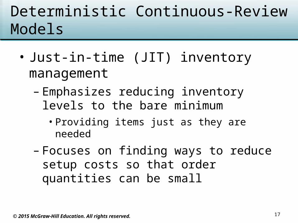
• Just-in-time (JIT) inventory management– Emphasizes reducing inventory levels to the
bare minimum• Providing items just as they are needed
– Focuses on finding ways to reduce setup costs so that order quantities can be small
17
© 2015 McGraw-Hill Education. All rights reserved.
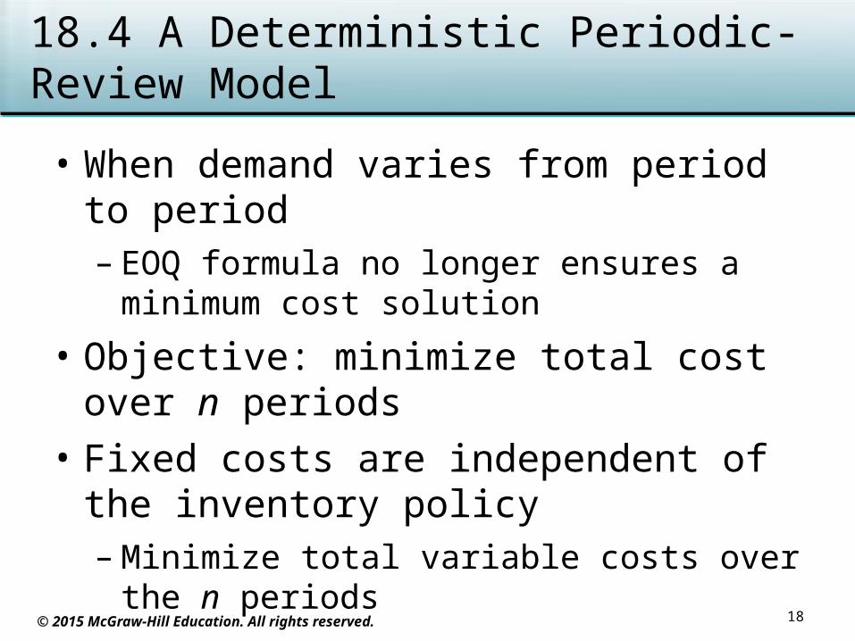
18.4 A Deterministic Periodic-Review Model
• When demand varies from period to period– EOQ formula no longer ensures a minimum
cost solution
• Objective: minimize total cost over n periods
• Fixed costs are independent of the inventory policy– Minimize total variable costs over the n
periods
18

© 2015 McGraw-Hill Education. All rights reserved.
A Deterministic Periodic-Review Model
• Example given on Pages 815-817 of the text
• An algorithm for an optimal inventory policy– An optimal policy produces only when the
inventory level is zero
19

© 2015 McGraw-Hill Education. All rights reserved.
18.5 Deterministic Multiechelon Inventory Models for Supply Chain Management
• Echelon– Each stage in a multi-stage inventory system
• Supply chain– Network of facilities that take raw materials
and transform them into finished goods at the customer
– Includes procurement, manufacturing, and distribution
20
© 2015 McGraw-Hill Education. All rights reserved.
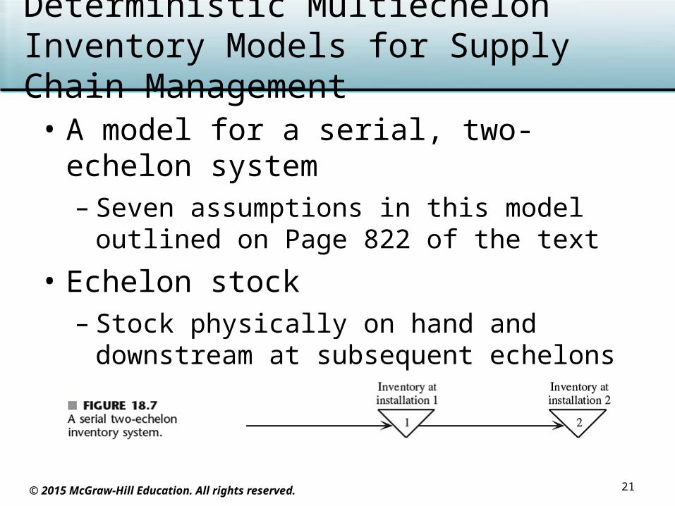
Deterministic Multiechelon Inventory Models for Supply Chain Management
• A model for a serial, two-echelon system– Seven assumptions in this model outlined on
Page 822 of the text
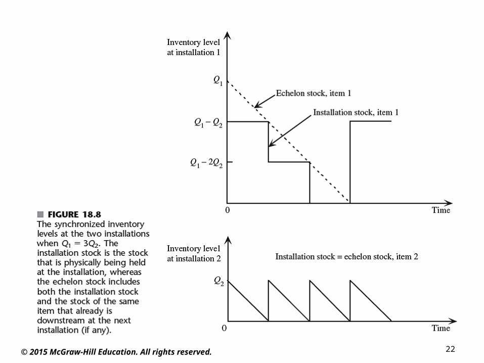
• Echelon stock– Stock physically on hand and downstream at
subsequent echelons
21
© 2015 McGraw-Hill Education. All rights reserved.
22

© 2015 McGraw-Hill Education. All rights reserved.
Deterministic Multiechelon Inventory Models for Supply Chain Management
• Optimizing the two installations separately– A flawed approach
– Choosing order quantities for installation 2 must account for the resulting costs at installation 1
• Optimizing the two installations simultaneously– Correct approach
– Process outlined on Page 826-827 of the text
23
© 2015 McGraw-Hill Education. All rights reserved.
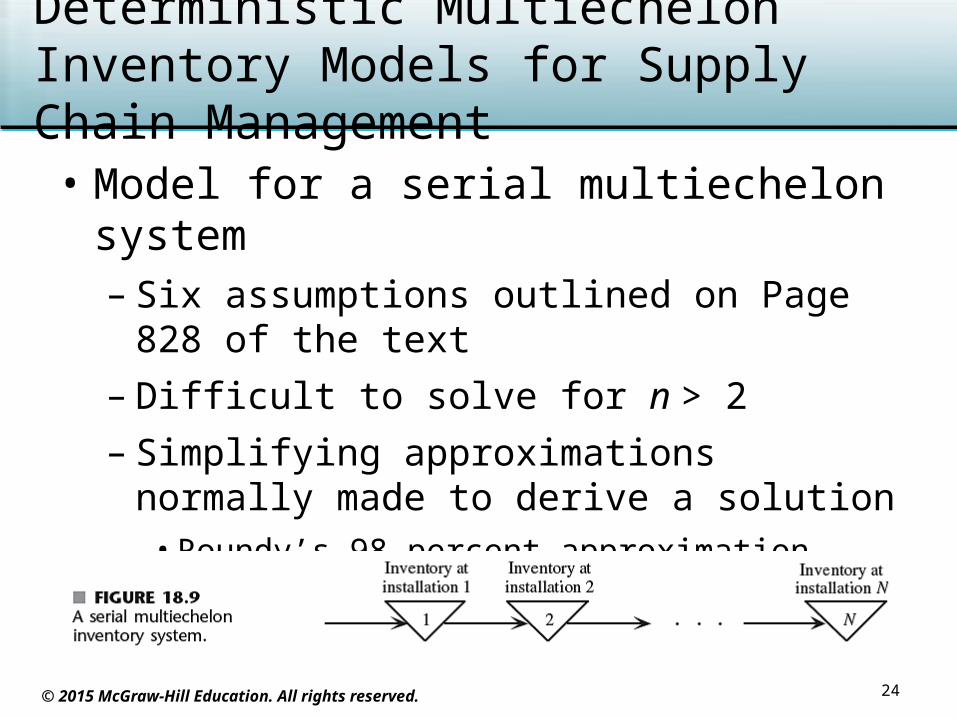
Deterministic Multiechelon Inventory Models for Supply Chain Management
• Model for a serial multiechelon system– Six assumptions outlined on Page 828 of the
text
– Difficult to solve for n > 2
– Simplifying approximations normally made to derive a solution
• Roundy’s 98 percent approximation property
24
© 2015 McGraw-Hill Education. All rights reserved.
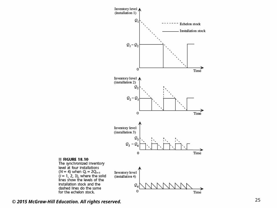
25
© 2015 McGraw-Hill Education. All rights reserved.
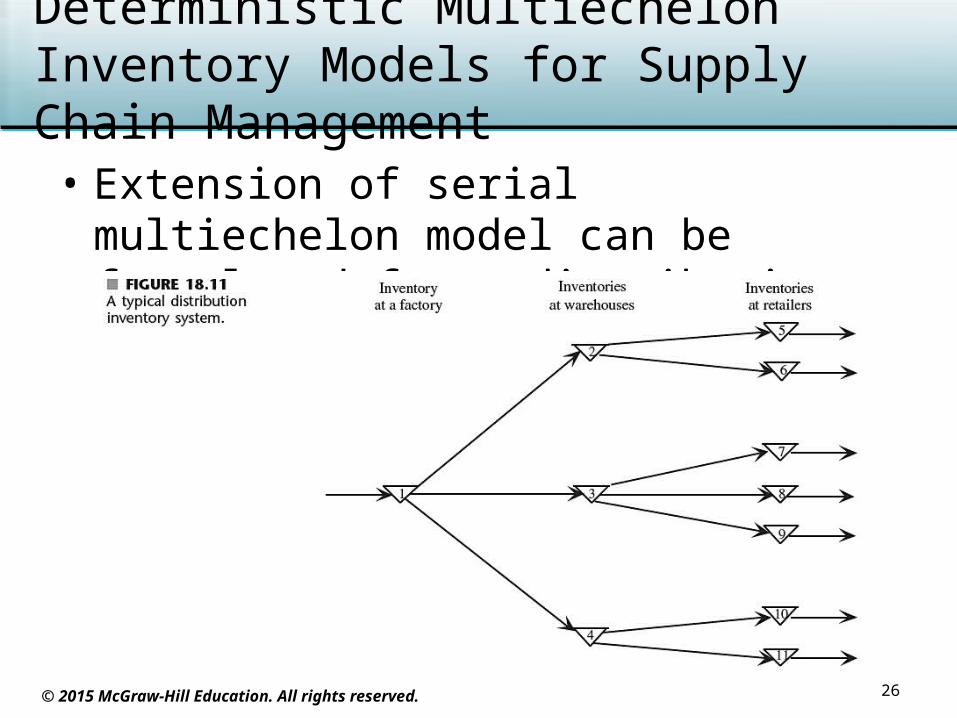
Deterministic Multiechelon Inventory Models for Supply Chain Management
• Extension of serial multiechelon model can be formulated for a distribution system
26

© 2015 McGraw-Hill Education. All rights reserved.
18.6 A Stochastic Continuous-Review Model
• Traditional method: a two-bin system– All units for a particular product held in two
bins
– Capacity of one bin equals the reorder point
– Units first withdrawn from the other bin
– Emptying second bin triggers a new order
• Newer approach: computerized inventory systems– Current inventory levels are always on record
27

© 2015 McGraw-Hill Education. All rights reserved.
A Stochastic Continuous-Review Model
• Inventory system based on:– Reorder point, R
– Order quantity, Q
• Inventory policy: whenever inventory drops to R units, place an order for Q more units
• Ten model assumptions outlined on Page 839 of the text
28
© 2015 McGraw-Hill Education. All rights reserved.
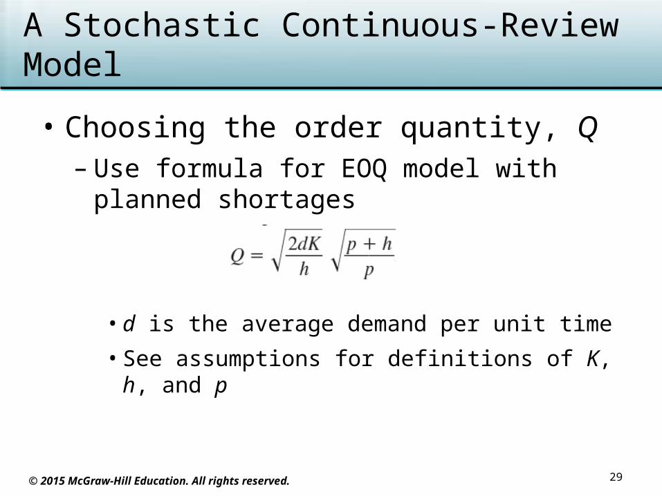
A Stochastic Continuous-Review Model
• Choosing the order quantity, Q– Use formula for EOQ model with planned
shortages
• d is the average demand per unit time
• See assumptions for definitions of K, h, and p
29

© 2015 McGraw-Hill Education. All rights reserved.
A Stochastic Continuous-Review Model
• Choosing the reorder point, R– Based on manager’s desired level of service
to customers
• Alternative measures of service level– Probability that a stockout will not occur
between the time an order is placed and when the order quantity is received
– Average number of stockouts per year
30
© 2015 McGraw-Hill Education. All rights reserved.
A Stochastic Continuous-Review Model
• Alternative measures of service level – Average percentage of annual demand that
can be filled immediately
– Average delay in filling backorders when a stockout occurs
– Overall average delay in filling orders• Where delay without a stockout is zero
31

© 2015 McGraw-Hill Education. All rights reserved.
A Stochastic Continuous-Review Model
• Measure 1 is most convenient to use
• Procedure for choosing R under service level measure 1– Choose L
– Solve for R such that
• Example given on Page 841 of the text
32
© 2015 McGraw-Hill Education. All rights reserved.
18.7 A Stochastic Single-Period Model for Perishable Products
• Stable product– Will remain sellable indefinitely
• Perishable product– Can be carried in inventory only a certain
amount of time
– Single period model is appropriate in this case
– Types of perishable products• Newspapers, flowers, seasonal greeting cards,
fashion goods, and airline reservations for a particular flight
33
© 2015 McGraw-Hill Education. All rights reserved.
A Stochastic Single-Period Model for Perishable Products
• Seven assumptions of the model– Given on Pages 846-847 of the text
• Analysis of the model with no initial inventory and no setup cost– Simplest case to consider
– See Pages 847-849
– Application to the bicycle example
• Analysis extends to include setup cost and initial inventory levels
34

© 2015 McGraw-Hill Education. All rights reserved.
18.8 Revenue Management
• Airlines started using revenue management in the late 1970s
• Overbooking– One of the oldest and most successful
revenue management practices
• Revenue management in the airline industry today– Pervasive, highly developed, and effective
35

© 2015 McGraw-Hill Education. All rights reserved.
Revenue Management
• Model for capacity-controlled discount fares– Decision variable: inventory level that must be
reserved for highest-paying customers
– Key to solving: marginal analysis
• An overbooking model– Choose overbooking level to maximize profit
– Shortage cost (denied-boarding cost) is incurred if overbooking level is too high
36

© 2015 McGraw-Hill Education. All rights reserved.
18.9 Conclusions
• Models presented in this chapter illustrate the general nature of inventory models
• EOQ models have been widely used
• Stochastic single-period model is appropriate for perishable products
• Multiechelon inventory models play an important role in supply chain management
37