© 2010 Eric Sam Nortrup

CFD STUDY OF DIFFUSER GEOMETRY EFFECTS ON DIFFUSER AUGMENTED WIND TURBINE PERFORMANCE

BY

ERIC SAM NORTRUP

THESIS

Submitted in partial fulfillment of the requirements for the degree of Master of Science in Mechanical Engineering

in the Graduate College of the University of Illinois at Urbana-Champaign, 2010

Urbana, Illinois

Advisor:

Professor Jimmy Hsia

ii

ABSTRACT

This thesis aims to explore the performance limits of diffuser augmented

wind turbines. Many studies of this topic have been performed in the

past. Limiting assumptions and manufacturing concerns have forced the

majority of previous studies to stray away from finding optimal

performance in favor of economical construction. A momentum theory

exists that shows the Betz limit can be exceeded by diffuser augmented

wind turbines. In a multistage optimization study, geometry factors are

considered and compared based on resulting power coefficients. In the

final phase of the study a diffuser is chosen and compared to previously

designed and tested diffusers. The new diffuser is the first to consider

performance based not on rotor area, but on diffuser exit area. This

diffuser exceeds the Betz limit based on diffuser exit area without

considering the beneficial effects of blade tip vortices that have been

found in multiple real-world tests.

iii

ACKNOWLEDGMENTS

The author wishes to express sincere appreciation to Professors Hsia for

his assistance in the preparation of this manuscript and for agreeing to

work with a non-traditional, off-campus thesis project. In addition,

special thanks to David Shelander whose words of encouragement and

passion for continually learning and growing inspired this study. Thanks

also to Dr. Jack Yan who has always fully accommodated the

requirements of my graduate studies with a flexible work schedule. And

finally, thanks to my girlfriend and family who have helped me through

the sometimes trying process of earning my Master’s Degree.

iv

TABLE OF CONTENTS

List of Symbols ............................................................................................. vi Chapter 1: Introduction.................................................................................1

1.1. Wind Power Beginnings .............................................................2 1.2. Scope of the Research..................................................................4 1.3. Overview ......................................................................................6 1.4. Figures ..........................................................................................7

Chapter 2: Theory ..........................................................................................8 2.1. Theoretical Framework for Wind Turbines .............................8 2.2. DAWT Momentum Theory........................................................9

Chapter 3: Review of Literature .................................................................12 3.1. Physical Tests .............................................................................12 3.2. Analytical Studies......................................................................16

Chapter 4: Experimental Methods .............................................................17 4.1. Research Methodology .............................................................17 4.2. Data Collection ..........................................................................18 4.3. Test Setup ...................................................................................20 4.4. Testing Phases............................................................................21 4.5. Figures ........................................................................................29 4.6. Tables ..........................................................................................33

Chapter 5: Results and Discussion ............................................................34 5.1. Data Reduction ..........................................................................34 5.2. Straight Walled Diffusers .........................................................34 5.3. Curved Geometry Study ..........................................................36 5.4. Final Design Optimization Phase ............................................40 5.5. Discussion ..................................................................................41 5.6. Figures ........................................................................................43 5.7. Tables ..........................................................................................54

Chapter 6: Conclusion .................................................................................57 6.1. Recommended Future Studies.................................................58

v

References .....................................................................................................60 Appendix A: Turbulence Model Comparison .........................................63

A.1 Figures..............................................................................................64 Appendix B: Comparison to Previous Tests.............................................65

B.1 Bare Turbine.....................................................................................65 B.2 Grumman Diffuser ..........................................................................66 B.3 Auckland Diffuser ...........................................................................67 B.4 Figures ..............................................................................................68 B.5 Tables ................................................................................................72

vi

LIST OF SYMBOLS

a Axial Flow Interference Factor

Disc Area

Diffuser Area

Wake Area

Area Far Upstream

Drag Coefficient

Thrust Factor

Ambient Thrust Coefficient

Power Coefficient Based on Rotor Area

Power Augmentation

Specific Power Coefficient

Betz Limit

Wake Pressure Coefficient

F Force

L Characteristic Length

Pressure at Diffuser Exit

Pressure in Wake

Pressure Upstream of Rotor

Pressure Downstream of Rotor

Pressure Far Upstream

Pc Power Available

Pw Power of the Wind

Velocity at Disc

vii

Wake Velocity

Velocity Far Upstream

V Flow Velocity

Diffuser Exit Area Ratio

ν Kinematic Viscosity

Density

Exit Backpressure Ratio

dP Pressure Difference

Reynolds Number

DAWT Diffuser Augmented Wind Turbine

EAR Exit-Area-Ratio

HAWT Horizontal-Axis Wind Turbine

VAWT Vertical-Axis Wind Turbine

1

CHAPTER 1: INTRODUCTION

Wind power generation is a rapidly growing industry and an important

source of energy. Worldwide wind power capacity is currently over 158

GW [1]. It is estimated by industry experts that by the year 2014 this

capacity will be greater than 400 GW. In the United States more than 35

GW of wind power capacity are currently in service. This 35 GW only

makes up about 2% of the current US energy needs [1]. 2% is a

surprisingly small amount, but it also indicates that there is substantial

room for growth. In addition, rising oil prices and an unstable Middle

East are ensuring that alternative energies make their way into the

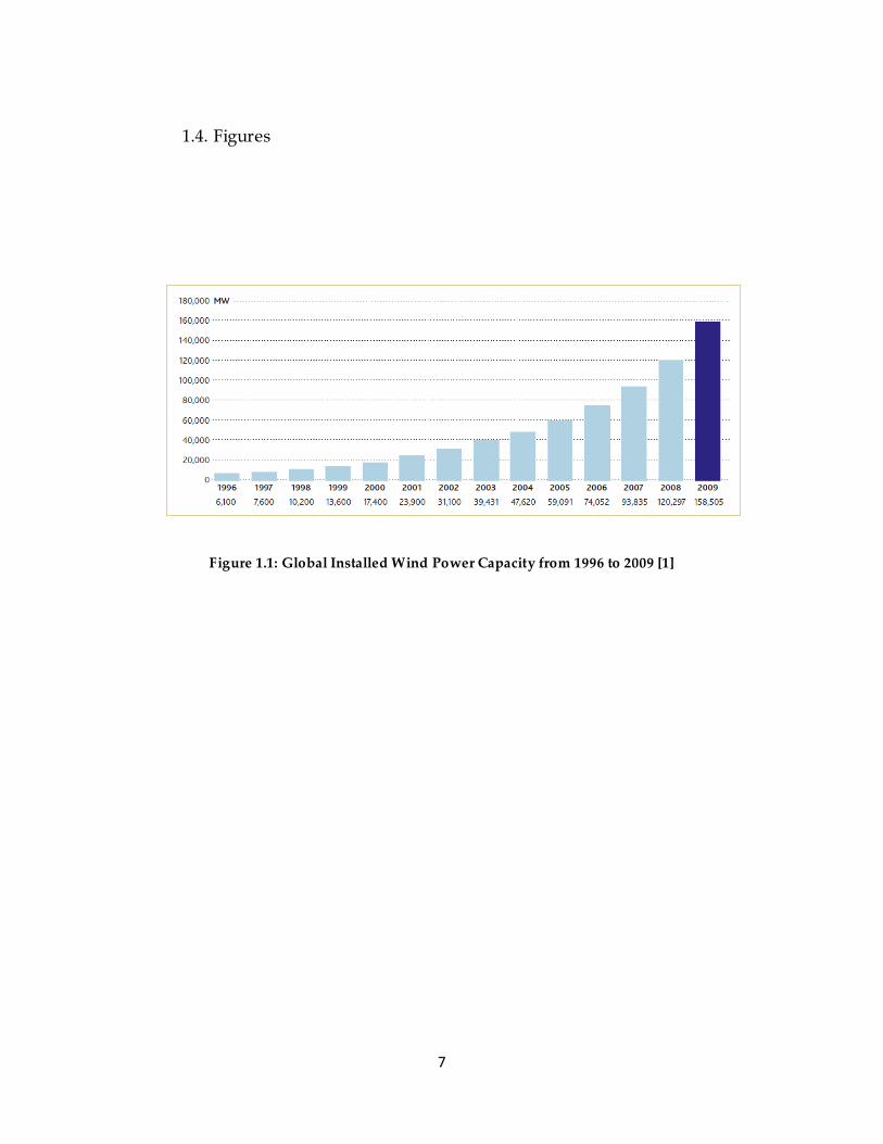
mainstream of energy production. Figure 1.1 shows the cumulative

installed capacity for wind power worldwide.

One limitation of wind power generation is the low kinetic energy of the

wind. While the average wind speed at a potential wind farm site is

critical, wind energy is, in general, a very diffuse energy. This is due to

the low density of air as compared to, for example, water, which is 800

times denser. In order to capture a significant amount of power and make

wind power more economically viable, wind turbine sizes have been

growing larger and larger. Current land based windmill farms have

turbines with diameters of around 100m. These have become so large that

they are becoming increasingly difficult to transport to an installation site.

2

The Betz limit 0.593 is the theoretical limit on the amount of energy a bare

wind turbine can collect. Great deals of research and development time

have been devoted to optimizing wind turbine blade designs. Mechanical

losses due to friction and drag result in real world performance lower

than this limit. The most efficient modern horizontal wind turbines

capture roughly 70 to 80% of this limit or 40 to 45% of the wind’s potential

energy.

1.1. Wind Power Beginnings

The use of wind power far precedes the invention of and subsequent

growing demand for electricity. The earliest windmills were literally

mills. In fact, the first wind mills were seen in ancient Persia and were

used to grind grains [2]. These first windmills could also be considered

the first augmented windmills. They were Savonius, or drag based

vertical axis wind turbines, VAWTs, that incorporate scoops or sails and is

partially contained in an outer structure that channels the wind [3]. From

this it is clear that the idea of increasing the energy density of wind is not

a new one.

Horizontal axis wind turbines or HAWTs later gained popularity in

Europe. They became widely used for grinding grain and pumping

water [3]. Since the first windmills there have been vast array s of designs

for increasing their power output. One of the more prominent methods is

3

the addition of a diffuser around or behind a conventional HAWT

creating a diffuser augmented wind turbine, DAWT. A Diffuser used to

augment an HAWT can create a large low pressure zone in the wake of

the turbine that pulls more air at higher velocity past the turbine. This

energy dense air that is passing through the diffuser and turbine has

increased kinetic energy and, therefore, the amount of energy captured by

the turbine can be significantly increased.

While this topic has been investigated numerous times, due to the

complex nature of the problem there has been limited success in

parametrically evaluating the features that impact effectiveness or

augmentation. There are, in fact, a great deal of parameters that can be

examined. One way to make a study more manageable is to set strict

limits on parameter variation. In many studies, the initial assumptions

and range limits have been so restrictive as to limit the potential for

augmentation. The current study is specifically targeting and attempting

to exceed the long established Betz limit based on diffuser exit area and

not rotor diameter. This is done by parametrically making geometry

changes to optimize a diffuser for a given cross-sectional area and length.

This thesis looks at diffuser geometry with limited initial restrictions in an

attempt to find the limits of attainable augmentation an d DAWT

efficiency.

4

1.2. Scope of the Research

1.2.1. Limitations of the study

Due to budget limitations this study is strictly performed through

computer simulation. A commercially available computational fluid

dynamics, CFD, code is used to simulate wind tunnel testing. Multiple

geometry factors are varied. Power coefficients and specific power

coefficients are compared as performance criteria. In addition pressure,

velocity, and thrust coefficient readings were taken to expose any possible

trends or critical correlations. In order to ensure accuracy and

comparability with previous studies, designs that were previously built

are analyzed and results are compared back to the empirical findings.

1.2.2. Unique Aspects

Many of the previous studies on this topic have incorporated very limiting

initial constraints. Admittedly, many of these constraints are necessary to

attempt to produce a cost effective and commercially viable end product.

Instead of focusing strictly on producibility and cost effectiveness, this

study focuses on optimizing power augmentation versus diffuser exit

area. It is the assertion of the author that understanding the limits of

performance and effects of geometry changes will be a valuable

engineering design reference. It will allow for a more informed decision

making process when manufacturability or production cost reduction

choices must be made. Some of the most prominent prior designs are

5

examined in an attempt to explore the bounds of augmentation in a CFD

format. There are two previous studies, in particular, that have had some

level of success in demonstrating increased performance level. These

designs are to this date the most efficient at augmenting a wind turbine

based on diffuser area. Some of the assumptions made during these

studies are loosened to explore diffuser augmentation possibilities or

limitations.

1.2.3. Impact of Study

The structural support associated with mounting a land based DAWT

makes the design cost prohibitive [4]. Mounting a DAWT 150 to 200 ft in

the air, while possible, would require massive structural support. This is

due to the much higher drag coefficient of the diffuser as compared to a

feathered traditional turbine of similar area. It would require a very

robust support structure in the case of extreme winds. One area where

this design could be highly effective is in ocean based wind farms. Due to

the lack of obstacles and lower turbulence levels, ocean based wind

turbines can be mounted much nearer to the water surface. In addition,

the underwater supports of an ocean based wind farm could be linked to

add structural integrity that would be an eye sore for a land based wind

farm.

Another area of potentially profitable exploitation of DAWTs is in

building top applications. This is, again, due to the fact that there are

6

fewer obstructions and therefore less hub height is required to capture

optimal wind flows. With the enhancements in performance made in this

thesis, the DAWT may be one step closer to successful commercializat ion.

1.3. Overview

The thesis is broken up into several chapters that contribute to different

aspects of the study. Chapter 2 discusses the theoretical background of

wind energy capture and DAWTs. It then goes on to discuss some of the

theory behind and reasons for adding a diffuser to the wind turbine.

Chapter 3 reviews previously published research and analysis. This

chapter looks at several prominent studies in the history and development

of the diffuser augmented wind turbine. Chapter 4 discusses the methods

used in the research that was completed in preparation for this thesis. It

describes the parameters examined and outputs collected in the various

stages of the study. Chapter 5 reviews the results of the research

described in Chapter 4. It presents a series of relationships between

geometry parameters and power augmentation. Chapter 6 summarizes

the findings in Chapter 5. It goes on to draw conclusions about the

diffuser augmented wind turbine based on these findings. The most

significant of the findings is successfully exceeding the Betz limit based on

diffuser exit area. The appendices present detailed information that

supports the finding discussed in the thesis. The appendices include the

presentation of a turbulence model comparison study and CFD analysis of

rotor disc theory and prior designs.

7

1.4. Figures

Figure 1.1: Global Installed Wind Power Capacity from 1996 to 2009 [1]

8

CHAPTER 2: THEORY

2.1. Theoretical Framework for Wind Turbines

Wind energy is collected by removing kinetic energy from passing wind.

This energy is turned into rotation when the wind produces a torque on

the turbine blades. The rotation is usually passed through a gearbox to

turn at the correct speed to operate a generator and produce a current.

The energy available from wind is given by

Pw = (2.1)

The mass of air passing through the rotor plane or disc can be thought of a

separate from the surrounding air. In this way air flowing through a

traditional horizontal axis wind turbine can be considered to be a stream-

tube [5]. Due to the conservation of mass and the decrease in velocity as

the air approaches and passes through the rotor disc, the disc area must

change with changing velocity. For conservation of mass to hold

(2.2)

The velocity slows as it approaches the turbine due to the increased

pressure near the obstruction of the rotor and the absorption of kinetic

energy by the rotor. In order for mass to be conserved, this slowing causes

the area of the stream-tube to increase as it approaches and passes

through the wind turbine. This means that the kinetic energy of the air

passing through the turbine is more diffuse than it is in the free stream.

9

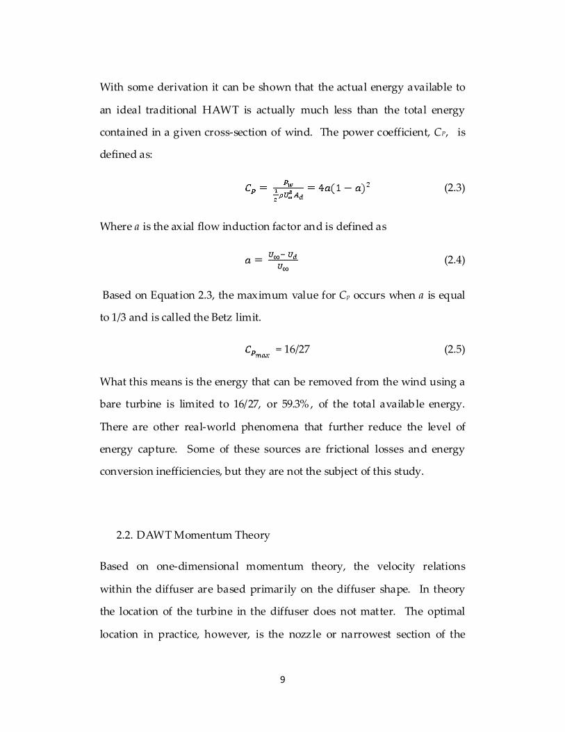
With some derivation it can be shown that the actual energy available to

an ideal traditional HAWT is actually much less than the total energy

contained in a given cross-section of wind. The power coefficient, CP, is

defined as:

(2.3)

Where a is the axial flow induction factor and is defined as

(2.4)

Based on Equation 2.3, the maximum value for Cp occurs when a is equal

to 1/3 and is called the Betz limit.

= 16/27 (2.5)

What this means is the energy that can be removed from the wind using a

bare turbine is limited to 16/27, or 59.3% , of the total available energy.

There are other real-world phenomena that further reduce the level of

energy capture. Some of these sources are frictional losses and energy

conversion inefficiencies, but they are not the subject of this study.

2.2. DAWT Momentum Theory

Based on one-dimensional momentum theory, the velocity relations

within the diffuser are based primarily on the diffuser shape. In theory

the location of the turbine in the diffuser does not matter. The optimal

location in practice, however, is the nozzle or narrowest section of the

10

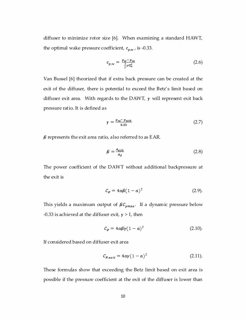
diffuser to minimize rotor size [6]. When examining a standard HAWT,

the optimal wake pressure coefficient, , is -0.33.

(2.6)

Van Bussel [6] theorized that if extra back pressure can be created at the

exit of the diffuser, there is potential to exceed the Betz’s limit based on

diffuser exit area. With regards to the DAWT, will represent exit back

pressure ratio. It is defined as

(2.7)

represents the exit area ratio, also referred to as EAR.

(2.8)

The power coefficient of the DAWT without additional backpressure at

the exit is

(2.9).

This yields a maximum output of . If a dynamic pressure below

-0.33 is achieved at the diffuser exit, > 1, then

(2.10).

If considered based on diffuser exit area

(2.11).

These formulas show that exceeding the Betz limit based on exit area is

possible if the pressure coefficient at the exit of the diffuser is lower than

11

-0.33 and flow separation does not occur. Some theorists have stated that

the limit of for a DAWT may be 89% or greater [7, 8]. will be

referred to as the specific power coefficient,

(2.12).

The goal of the current study is to maximize the specific power coefficient.

As previously shown this can be done by creating a low pressure zone at

the exit of the diffuser. The difficulty with this task is that separation

must be avoided for the theoretical results to be realized. This thesis will

focus on achieving this fully attached flow.

12

CHAPTER 3: REVIEW OF LITERATURE

Many studies have investigated methods and designs for augmenting

wind turbine performance with a diffuser. One of the first theoretical

papers on the topic was written in the 1950’ s and indentified the

potentially beneficial results of creating a low pressure zone behind a

traditional HAWT [9]. There was little interest in the idea until the 1970’s

oil crisis brought alternative energy to the forefront of discussions [10]. It

was at this time that several separate researchers began in-depth studies

of diffuser augmentation.

3.1. Physical Tests

Two prominent examples of the work done in the 1970’s, are the

Grumman Aerospace studies conducted by Foremann et al. [11, 12, 13, 14]

and the University of Negev study conducted by Ozer Igra [15]. These

investigations showed some promising results and were an important first

step in the development of DAWTs. Igra’s initial work involved wind

tunnel studies of multiple small scale diffusers. Mesh screens of different

solidity were used to simulate the resistance of a turbine and to examine

the potential power of the diffuser with varying turbine thrust factors, Ct.

(3.1)

13

Where p1 is the pressure just upstream of the rotor and p2 is the pressure

just downstream of the rotor.

The first generation shroud was 7 rotor diameters long with an 8.5 degree

diffuser angle. The resulting exit area ratio, EAR, was 3.5. Three different

bell-shaped inlets were used with this first diffuser. The results of this

wind tunnel testing showed impressive augmentation results of 2.5 to 3.0

times the performance of a bare wind turbine. The massive diffuser size

was totally impractical from a commercial standpoint and Igra proceeded

to a second generation short diffuser shroud. This second design used

had a length to diameter ratio, LTDR, of 3.64, and EAR of 2.0 with a

diffuser angle of 12.5 degrees. This design also incorporated 3 annular

rings with gaps between them to help prevent flow separation. These

rings also increased the exit area ratio to 10.0. The peak power

augmentation, Cp,Betz was 2.8 with 3 rings at a Ct of 0.22 [15].

(3.2)

As mentioned, around the same time, Foreman working for Grumman

Aerospace was conducting research on a different version of the diffuser

augmented wind turbine. This study focused on boundary layer control

and minimizing diffuser size [12]. Grumman's initial theoretical analysis

showed that optimization goals of large EAR, large velocity increase, and

a negative exit pressure. Being that Grumman’s goal was commercial

14

viability, they chose a moderate EAR in favor of lower cost. This study

examined a single skin boundary-layer control type diffuser [14]. The

boundary layer control device was various inlets between multiple

diffuser extending rings. A wide variety of straight section diffusers with

angles from 40 to 90 degrees were used. These diffusers had EARs from

1.28 to 4.94 [13]. Like Igra, Grumman used various mesh screens to

simulate turbines with thrust factors between 0.37 and 0.94. Studies of

ring slot height and overlap were conducted. In all over 150

configurations built and tested, but they all were base on the straight

diffuser of a conic profile. The final product of the Grumman study was a

60 degree diffuser that has a LTDR of 0.715 and an EAR of 2.78. The peak

augmentation, or Cp,Betz, of 2.3 was achieved with a rotor thrust factor of

0.55 in the baseline diffuser model [13]. Foreman concluded that the

DAWT was not economically competitive with traditional HAWTs [11,

14]. This lead to a period of inactivity on the subject until some

researchers from New Zealand decided to reexamine the subject.

In 1995 Vortec Energy Company bought the rights to some of Grumman’s

work and began an effort to commercialize the DAWT [16]. They teamed

with the University of Auckland in New Zealand to develop a 7.3m

prototype. In addition to this large scale prototype an extensive study

that incorporated theoretical, CFD, and wind tunnel development was

undertaken. This study resulted in several new findings and improved

results. The end result of the study was a diffuser with a short 0.48 LTDR

15

and a 3.0 EAR [9]. The resulting performance augmentation with respect

to the Betz limit was 1.73. Some of the conclusions Phillips arrived at

were: augmentation is maximized when air flow is directed radially at the

exit by having a large diffuser angle at the exit. Diffuser flaps were found

to be best when of width roughly 5% of exit diameter.

It was found that a constant area section in around the rotor was

unnecessary. The study made some promising steps forward in

developing a passive boundary layer control system. The study also

agreed with many previous researchers in finding that EARs over 3.0

would not provide an efficient increase in augmentation. While this study

showed a reasonable level of augmentation in the smallest diffuser size to

date it left some areas for improvement.

There was a significant discrepancy between power coefficient during

wind tunnel testing using the filter turbine and full scale testing with a

rotor in place. It was claimed that the reason for this discrepancy was the

beneficial effect of the blade tip vortices in mixing the inner and boundary

layer flows. While this effect is likely to have contributed to the difference

in augmentation, the higher Reynolds number associated with the large

scale tests have proved to be beneficial in other experiments [17].

16

3.2. Analytical Studies

A CFD study conducted in 1999 was the first to present results that

showed the Betz limit was approachable in relationship to the diffuser exit

area [18]. This study was conducted on a 10 degree slice of a cylindrical

wind tunnel. The test tunnel extended 5 diffuser lengths upstream and 10

downstream. In addition it had a radius of 10 diffuser lengths. A

NACA0015 airfoil shaped diffuser was used with a LTDR of 1.06 and a

EAR of 1.84 [18]. The inlet velocity was prescribed such that the Reynolds

number was 5 x 107. A Reynolds number this high would be represented

by a 42m rotor in a 10m/s wind with an 89m long diffuser. As later

discussed, in Chapter 5, higher Reynolds numbers yield significantly

increased CP values.

This setup resulted in a rotor plane velocity increase of 1.83 with no rotor

present. With a rotor present, the design showed CP results that reached

0.94 at a Ct of 0.80. This results in a CP,exit of 0.514, or 87% of the Betz limit.

This study is the first to show that the Betz limit is approachable based on

diffuser EAR. A down side of this study is the small EAR, large LTDR,

and very high Reynolds numbers. Later CFD design and analysis studies

have shown higher CP values, but when CP,exit is examined they fell short

[19, 20].

17

CHAPTER 4: EXPERIMENTAL METHODS

This study consisted of parametric research that was conducted using Pro

Engineer as a design tool and STAR CCM+, a commercially available CFD

program used for analyzing problems from heat transfer to supersonic

aircraft. The study was conducted in a multi-phase optimization

methodology; focusing on and identifying critical relationships in an

empirical study and comparing these back to previous literature findings.

4.1. Research Methodology

Since this study effort consists strictly of computer simulations, a standard

test fixture was designed based on the guidance of previous CFD studies

[17, 19]. The wind tunnel for this study was a cylinder that was 15 rotor

diameters long and 10 rotor diameters wide. The large size was chosen to

avoid having faulty data due to high levels of tunnel blockage. In fact, the

large size of the test tunnel meant that the diffusers considered in this

study only presented a 2-3% blockage.

Most of the designs considered were axis-symmetric in nature, and a 2-D

model may seem adequate. This type of 2-D model would have saved a

significant amount of computing time. If a 2-D model had been used,

however, 3-D effects of vortices would be neglected. The decision to go

with a 3-D study allowed the addition or study of vortex generating

18

devices and other variable angle slot or inlets. 3-D as the test wind tunnel

is, it did not require that the entire 360 degrees be captured. A 45 degree

slice of the tunnel was chosen to save on computing time, see Figure 4.1.

The wedge wind tunnel was meshed using the STAR CCM+ polyhedral

mesher, see Figure 4.2. The walls of the 45 degree slice of wind tunnel

were modeled as slip walls or walls that impart no shear stress on the air.

4.2. Data Collection

In order to isolate diffuser design, rotor design and optimizat ion are not

considered in this study. Instead the rotor is represented with a porous

media region. The region is assigned a predetermined resistance using an

iteration based table. The pressure differential from the inlet to outlet of

the porous region in conjunction with the velocity across the porous

region is used to establish the potential for energy collection.

Several pieces of data were collected with each diffuser design that was

analyzed. The inlet velocity for the wind tunnel was pre-defined for the

testing in this study. The area-average velocity of the air at the front face

of the rotor disc was monitored. Area-averaged pressure readings were

taken at the front and rear face of the simulated rotor. The difference in

pressures from these two planes is used to arrive at a pressure drop across

the turbine. In the final phase of the study, force exerted on the shroud

was recorded with varying turbine thrust factors. This information can

19

later be used for structural and extreme wind loading calculations. Varied

rotor thrust factors, Ct, were tested for each diffuser configuration. The

resulting pressure difference and velocity for each unique diffuser and

turbine was then used to arrive at a power coefficient.

(4.1)

The use of a range of turbine thrust factor settings allowed for the

identification of an optimal turbine design for any given diffuser, see

Table 4.1.

The meshed models contained from 60,000 to 100,000 cells. On average,

500 iterations of the solver were required for convergence of a stable

solution for a given set of inputs. To ensure convergence, simulations

were set to run to 1000 iterations per rotor thrust factor setting. This

iteration buffer allowed less stab le solutions to run through a series of 8 to

10 different thrust factors without a human monitor. Setting the

simulation to automatically step through thrust factors allowed 8-12 hour

simulations to be run overnight to avoid unnecessarily tying up the

limited number of available software licenses. At the end of a simulation

run, data was exported along with velocity and pressure difference plots

for verification of convergence of monitored parameters.

20

4.3. Test Setup

Design geometries for diffusers were constructed using Pro Engineer

Wildfire 3.0 CAD softwar e. They were then exported as a universal .STP

file that is compatible with STAR CCM+ and many other analytical tools.

The geometry was then imported to STAR CCM+ as a group of connected

surfaces. Each unique diffuser geometry was imported into the 45 degree

wind tunnel. The various surfaces of the diffuser were then combined to

form a single region, as defined in STAR CCM+. A simple Boolean

subtract was then performed to subtract the portions of the air from the

test wind tunnel that were intersected by the diffuser. In this way the inlet

and other boundary conditions were shared between different analysis

models. This also allows monitored outputs within the rotor and air

continuums to be setup in a shared test setup file. The setup file also

contained meshing parameters, thrust factor tables, and inlet velocities.

The analysis models were divided into air and rotor volumes with the

diffuser components being a represented as void in the air volume. A

hybrid polyhedral meshing algorithm was used to mesh the air and rotor

regions. The typical number of cells for a simulation was between 60,000

and 100,000. The simulation was setup as a 3-D stationary, steady state,

ideal gas analysis. The turbulence model used was the Averaged Navier-

Stokes method using K-Epsilon with realizable K two layer y+ wall

treatment.

21

4.4. Testing Phases

There were three separate phases of design and analysis that were

completed. The phases consisted of straight walled diffusers, curved

diffusers, and diffuser optimizat ion.

4.4.1. Straight Walled Diffusers

The initial phase of testing involved a basic characterizat ion of some gross

geometry parameters. In order to isolate the effects of various geometric

variables it was decided to hold the EAR and LTDR constant for the first

set of diffusers. As previously discussed, it was assumed that EARs over

3.0 would be difficult to eliminate boundary layer separation in. For this

reason the EAR was set at 3.0 and LTDR was set at 1.0. All the diffusers

used the same inlet profile. This was a single radius curve that had an 80

degree angle from diffuser center line to the opening at 1.09 times the

rotor diameter. This bell shaped inlet had an area 1.2 times that of the

turbine or diffuser throat. This initial inlet size was based on multiple

resources [6, 9, 15]. The diffusers contained a constant cross-section area

around the turbine followed by a straight walled diffuser, see Figure 4.3.

The variables for this phase of the investigation were diffuser half angle,

presence of slats, the presence of vortex generating tabs, and the presence

of an outer skin on the diffuser. Table 4.2 summarizes the different

geometry configurations analyzed.

22

Designs with 22.5, 30, 45, and 50 degrees were examined. In order to

maintain the 1.0 LTDR, the constant area section of the diffusers varied in

length. The 50 degree diffuser was of a stepped nature. The 50 degree

diffuser included a 22.5 and 36 degree section.

Vane-type vortex generating tabs, similar to those used on small aircraft to

delay separation and stall, were placed just upstream of flow separation

sites on the inside of the diffusers. This was done in an attempt to identify

any effects of the vortex mixing on boundary layer separation control and

more importantly power augmentation [20]. The vortex generator pairs

were of the vane-type and added in pairs as described in a paper by

Logdberg et al. [21].

To look at the potentially beneficial effects of injecting high energy

exterior flow into the low energy boundary layer inside the diffuser, the

diffusers were broken into multiple sections in some cases. These slats

that were created, with the breaking up of the diffuser into sections, were

examined as a potential method for delay of separation. In addition, an

outer skin was place around some diffusers to create a pressurized

chamber from air was injected into the slats. Overall, these designs were

simple to modify and served as a good format to setup analysis

parameters and verify analysis methods.

23

4.4.2. Curved profiles

The first phase of the study allowed for some basic flow effects to be

observed. The second phase of this study built off the extensive work

performed by researchers for Grumman Aerospace and the University of

Auckland [9, 13]. The first step was to accurately model the diffusers used

in these studies and replicate their results. This proved fairly difficult as

neither dimensional drawings nor clearly defined construction details

were presented in the Grumman or Auckland papers. The diagrams

presented in the papers were of generally poor quality and the low

resolution of the diagrams made accurate measurement difficult. In any

case, the geometries were modeled in Pro Engineer as accurately as

possible. The size of the slats and material thickness for the various

models had to be assumed. A number of similar geometries were

evaluated that produced results comparable with the findings in the two

studies. These designs were evaluated with the same test wind tunnel as

the other diffuser designs described in this thesis. The details and results

of these simulations can be found in Appendix B. To date the Grumman

study has demonstrated the best specific power coefficient based on

overall size of the diffuser although there have been questions about the

validity of some of the results [9]. Due to the limitations of straight

walled designs the diffusers in this phase the study used curved walls and

slats similar to the Auckland design.

24

One of the major contributors to the enhanced performance of this style of

diffuser is the inclusion of slats or annular gaps between the successive

rings of the diffuser. These gaps in combination with a curved profile

proved to significantly delay boundary layer separation; even with much

larger included angles than those found in the initial phase of the study.

The delay in separation is due to the high energy external flow increasing

the energy of the boundary layer air. These slats have been used in

airplane wings for many years and first showed up related to DAWTs in

the research of Igra and Foreman in the late 1970’s [13, 15]. The

parameters that were examined in this phase of the study were LTDR,

EAR, exit angle, ring gap, ring overlap, ring number, inlet size, multiple

skins, wind speed, an d scale.

LTDR was varied from the very short 0.48 of the Auckland diffuser to

0.83. This range, while much smaller than some previous studies,

adequately encompassed the range of efficient and cost effective sizes. It

also showed valuable trends on the optimal LTDR.

Exit area ratio was varied for this family of curved diffusers. The base

EAR of 3.0 was the used for initial diffusers. Since separation was

observed in all variations of the 3.0 EAR diffusers, it was decided to

progressively decrease the exit area while maintaining a similar curve

25

profile. EARs of 3.0, 2.75, 2.5, 2.35 and 2.0 were investigated. It was

expected that the power coefficient would decrease with decreased EAR.

The item of interest, and the unknown, was how the specific power

coefficient would change with EAR. The intention was to see if the

diffuser became more efficient with decreased diameter.

The Auckland study reported that the optimal diffuser included angle was

55 degrees [9]. This may have been the case for the extremely short

diffuser that was used in that study. When the LTDR was allowed to be

increased, it opened up the possibility to have a smaller included angle on

the diffuser. The exit angle for the diffusers used in this study phase

varied from 45 to 60 degrees.

Annular gaps between sections of the diffusers were present in all of the

phase two designs. The ring gap, or radial gap between each consecutive

diffuser ring, was the same for each ring in a given diffuser geometry.

This common gap size was varied from 0.58% to 0.83% of the rotor

diameter. Ring overlap, or the linear distance that each ring over lapped

the previous one, was varied as well. The ring overlap was varied from

0.25% to 2.0% of the rotor diameter. The idea being that there must be a

balance between guiding and focusing the flow and reducing the flow due

to viscous drag effects. Ring number was varied from 3 to 5 rings. The

Auckland diffuser that the profiles for this study were based on had an

outer surface or scoop that created a pressurized region that fed into the

26

boundary layer control slots. In this phase of the study diffuser profiles

were compared with and without an outer scoop.

Wind speed and scale were varied over a practical range. Performance at

wind velocities of 2, 5, 8, and 16m/s were used. For size variation, 4.6m

and 30.5m diameter rotors were used. In effect the same factor was being

varied for either case. The real reason for a performance change with

variation in these parameters was the fact that the Reynolds number was

being varied with different velocity and characteristic length parameters.

(4.2)

For this reason, only the velocity variation results are presented in

Chapter 5. The Reynolds numbers for the simulations in phase 2 varied

from 2.5 x 106 to 3.2 x 107. The higher Reynolds number flow is more

turbulent and the viscous effects at boundary layer have less impact on

the mainstream flow.

4.4.3. Optimizat ion study

After the phase two data was collected and summarized several trends

were found. Observing these trends and relationships, a phase three

study was conducted in an effort to exceed the Betz limit. While it was

clear that performance increase with increased Reynolds number, the

rotor size for this phase was held at a modest 4.6m. In addition the wind

27

velocity was held at 5 m/s. With this noted, it should be clear that the CP

results of this phase of testing could be improved by increasing rotor scale

or wind velocity. In this optimizat ion phase of the study the LTDR was

re-assessed based on an optimal EAR identified in phase two, see Figure

4.4. This phase of the study varied the length of the diffuser to identify an

optimal length and to collect the data that would be required to make

informed engineering decisions about size and structure tradeoffs.

A diffuser with a 50 degree half angle exit and an EAR of 2.5 was chosen.

The diffuser had an inlet area equal to 1.2 times the rotor area. The

diffuser was broken up into multiple sections. The base diffuser body

including the inlet section was 0.39 times the rotor diameter. The exit half

angle of the base diffuser was 28 degrees. The blade tip gap at the

narrowest section of the diffuser was 1.0% of the rotor diameter. The base

diffuser body was followed by 4 rings. The rings got progressively

shorter with larger diameter. The lengths of the rings were 10.4%, 8.8%,

7.1%, and 5.4% of the rotor diameter. Each ring increased the exit angle by

another 6.5 degrees for a 50 degree angle at the exit of the final ring. The

gap between each ring was 0.78% of the rotor diameter and the overlap

was 0.92% of the rotor diameter. The total LTDR for the initial diffuser

with rings was 0.58. Based on this rotor an investigation of LTDR, ring

gap, and ring overlap was conducted.

28

The ring gap size and ring overlap were varied plus and minus 10% from

the baseline geometry. The LTDR was varied from 0.5 to 0.78. This was

varied primarily by changing the length of the base diffuser. At the

extremes, the base diffuser exit angle had to be adjusted to maintain ring

length and angles. The overall exit half angle of 50 degrees was

maintained for all the variations. In addition no changes to the inlet side

of the diffuser were made.

4.4.4. Final Design

After the findings of the optimization phase of the study there was one

clear choice for the optimal diffuser. The final diffuser design had an EAR

of 2.52 and a LTDR of 0.72, see Figure 4.5. This diffuser was re-analyzed

to capture wind force data. In addition some additional post-processing

steps were conducted to compare the results back to theoretical works on

the topic of DAWTs. This diffuser was also used for a turbulence model

sensitivity study, Appendix A.

29

4.5. Figures

Figure 4.1: Screenshot of the 45 degree Test Wind Tunnel in STAR CCM+

Figure 4.2: Screenshot of Meshed Surface of a Diffuser and Rotor Model in STAR CCM+

30

Figure 4.3: 22.5 degree Diffuser from Phase One Testing

31

Figure 4.4: Diffuser Profiles used in Optimization Phase LTDR Study

32

Figure 4.5: Profile of the Best Performing Diffuser from Phase Three Testing

33

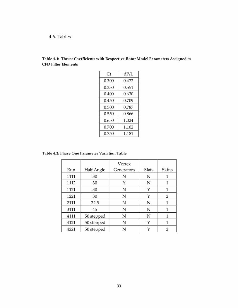
4.6. Tables

Table 4.1: Thrust Coefficients with Respective Rotor Model Parameters Assigned to CFD Filter Elements

Ct dP/L 0.300 0.472 0.350 0.551 0.400 0.630 0.450 0.709 0.500 0.787 0.550 0.866 0.650 1.024 0.700 1.102 0.750 1.181

Table 4.2: Phase One Parameter Variation Table

Run Half Angle Vortex

Generators Slats Skins 1111 30 N N 1 1112 30 Y N 1 1121 30 N Y 1 1221 30 N Y 2 2111 22.5 N N 1 3111 45 N N 1 4111 50 stepped N N 1 4121 50 stepped N Y 1 4221 50 stepped N Y 2

34

CHAPTER 5: RESULTS AND DISCUSSION

5.1. Data Reduction

Each diffuser test was run for 1,000 iterations at each rotor thrust factor.

The resulting data set consisted 10,000 data points that summarized dP,

Velocity, and various residuals. In order to get meaningful and

comparable information from these values, a data point well after solution

stabilizat ion was chosen. The sample value was typically taken after 950

iterations despite the fact that stabilizat ion occurred earlier in most cases.

The comparable output was Cp.

5.2. Straight Walled Diffusers

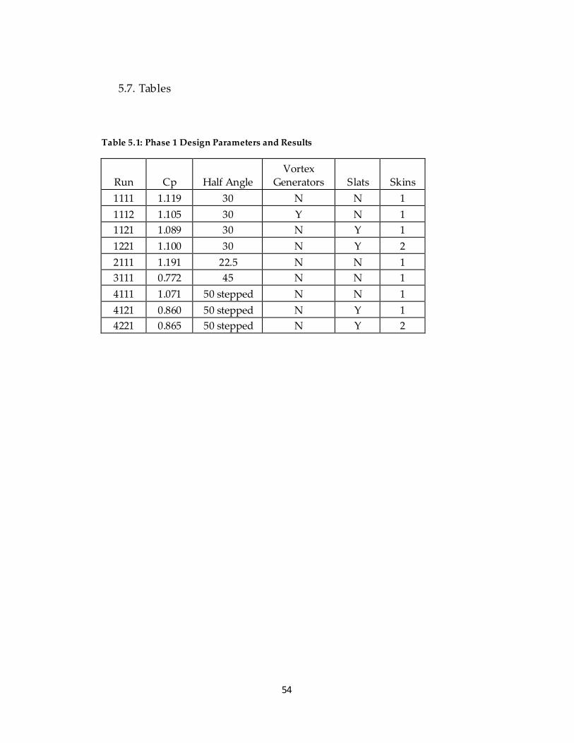
The first phase of the study yielded very dismal results, see Table 5.1.

Admittedly, this phase of the study more of a familiarizat ion exercise and

was not really intended to perform well. All of the straight walled

diffusers showed some degree of separation of the flow from the inner

edge of the shroud. The best performer was the 22.5 degree diffuser,

which only showed separation on the final 30% of the inner surface of the

diffuser. This was expected, as the recommended maximum angle to

avoid separation in a sub-atmospheric environment is 8-10 degrees [15].

The 45 degree diffuser showed a massive separation and recirculation

zone in the downwind region which reduced the mass flow of air through

35

the diffuser. The highest level of Cp was only 1.19, see Figure 5.1. The

peak Cp was found with Ct of the rotor set at 0.75.

The placement of tabs on various locations along the inner surface of the

diffuser and outer surface of the hub was evaluated. The best performing

location proved to be placing the vortex generating tabs on the inner

surface of the diffuser just upstream the point of boundary layer

separation. The vortex generators resulted in increased mixing of the high

energy inner flow and lower energy boundary layer. In this case,

however, the gross effect was the reduction of the mass flow through the

diffuser despite delayed separation, see Figure 5.2. It appears that the

additional drag from the vortex generators overpowered the beneficial

effects of the boundary layer mixing and can be attributed for this

reduction in power output. With this discovery, the vortex generator tab

design parameter was ruled out for the future phases of the study.

The addition of annular gaps or slats in the diffuser was investigated. The

gaps did not provide the boundary layer control that was expected based

on previous works. In this case, the addition of gaps resulted in a clear

decrease in power output, see Figure 5.3. This is thought to be the result

of non-optimal gap and overlap parameters. In addition to the slats, the

addition of an outer skin was evaluated. The addition of an outer skin

showed a modest increase in power output, see figure 5.4.

36

As the initial intention of this study was to build a prototype diffuser and

test it in a wind tunnel, these phase one diffusers were designed for a

rotor only 0.35m in diameter. At this small scale the viscous effects of air

play a much larger role on performance than they would on a more real-

world sized diffuser. The low Reynolds number air flow showed

significantly lower performance than later simulations that were

conducted. A larger version of the 22.5 degree diffuser was analyzed for a

comparison of results between these small wind tunnel-scaled models and

a larger scale private use or utility scale model. This larger model showed

a 25.2% improvement in CP. Later stages of testing were conducted on a

diffusers designed for a 4.6m diameter rotor. This larger size, while still

not equal, showed results that were more comparable with industrial

sized rotors.

5.3. Curved Geometry Study

As mentioned this phase of the study moved to a 4.6m rotor diameter.

The general geometries were of a curved nature roughly based off of

extended versions of the Auckland diffuser study [9]. A summary of the

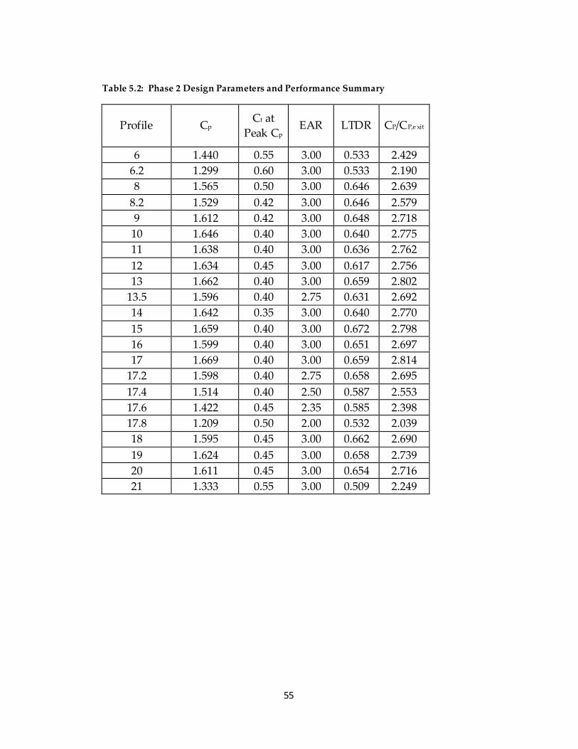
results can be found in Table 5.2.

37

5.3.1. Length to Diameter Ratio

LTDR showed a very significant contribution to the CP of the diffuser, see

Figure 5.5. The shorter diffusers showed high levels of separation at the

rear-most portion of the diffuser. The shorter diffusers also produced a

wider peak CP. This is probably due to the fact that as separation occurred

any potentially peak performance region was reduced resulting in a

broader CP versus Ct curve with a lower peak. The longer diffusers

showed a significant peak in the lower Ct zone from 0.25 to 0.35. The

longer the diffuser, the higher and more narrow banded this peak zone

became. This phase of the study showed a roughly linear relationship

between LTDR and Cp. Since there were still signs of separation at the

longest LTDR in this study, the range should have been extended to

expose the relationship in a fully attached flow. This was noted and

addressed in the later optimizat ion phase of the study.

5.3.2. Exit Area Ratio

Exit area played a very large role in the power coefficient. While this

result was expected, there were other interesting findings that resulted.

The CP increased with increasing EAR. The relationship between these

values did not show a linear increase, it resulted in a curve with

diminishing returns as the EAR increased, see Figure 5.6. This indicated

that perhaps the more appropriate value to look at would be CP,exit as EAR

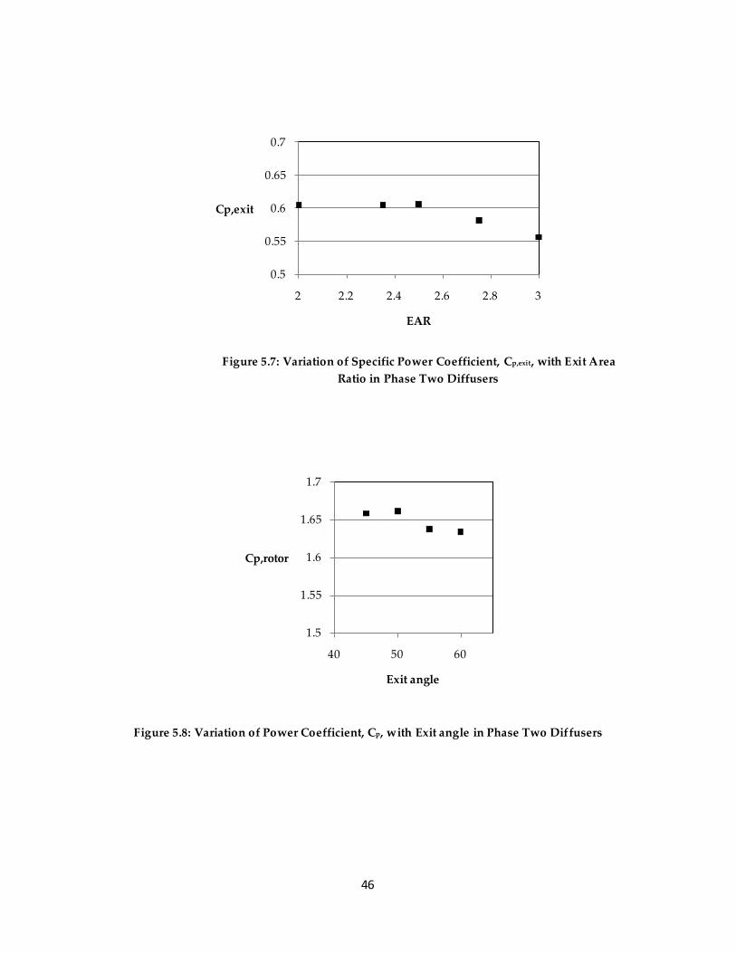
was varied, see Figure 5.7. Plotting these two values against each other

resulted in a clear break point and a potentially optimal value. As the

38

EAR decreased from 3.0 to 2.5, CP,exit increased from 0.55 to 0.61. This was

a 10 % increase in efficiency of the diffuser. More importantly this

reduction in EAR from the originally selected value resulted in a diffuser

that was giving a value of power coefficient higher than the Betz limit for

its given shroud diameter. This is the first diffuser to yield results that

exceed the Betz limit when compared to diffuser diameter.

5.3.3. Exit Angle

Exit Angle results showed that an important balance must be met. On one

hand, larger diffuser exit angles have to potential to create a wider low

pressure wake downwind of the diffuser. However, the larger diffuser

angles in this study resulted in separation of the interior flow from the

inner surface of the diffuser. This separation caused a recirculation zone

which caused a collapse of the potentially large low pressure wake from

the large included angle. In this study a 45 to 50 degree diffuser

performed marginally better, 1.6%, than the 55 and 60 degree diffusers,

see Figure 5.8.

5.3.4. Wind Velocity and Rotor Scale

Varying the wind speed and scale of the diffuser had the same basic

effects on the fluid dynamics of the analysis. Both varied the Reynolds

number. From the results in this study, increased Reynolds numbers led

to increased CP due to a reduction in shear forces imparted on the air flow.

39

The wind speed was varied from 2m/s to 16 m/s. The resulting range of

Reynolds numbers ranged from 2.5 x 106 to 3.2 x 107. Over this range, the

power coefficient showed a 3.5% increase from the lowest to highest wind

speeds, see Figure 5.9. The scaling effects were not explored in more

depth since the general trend was established by varying the velocity.

5.3.5. Ring Gap, Ring Overlap, Ring Number, and Inlet Size

Each of these parameters appeared to each show an optimal zone. While

the effects of being slightly off of the optimal values may have been small,

without the study of these factors a performance change of over 10% may

have been overlooked. Varying the inlet diameter by plus and minus 10%

only resulted in a 2.8% variation in the observed CP, see Figure 5.10. This

agrees with some previous works that stated inlet ratio optimizat ion was

not as critical as other geometry effects in producing enhanced power [6].

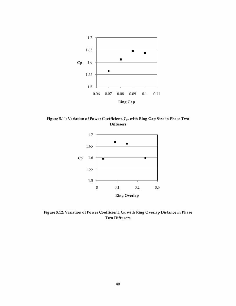
The same relationship was found with the ring gap. Ring gap was varied

in 0.08% of the rotor diameter increments from 0.58% to 0.83% of the rotor

diameter while the ring overlap was held constant at 1.25% of the rotor

diameter. CP levels varied by 5.1% for a ring gap variation over the range

mentioned, see Figure 5.11. The optimal value was found to be 0.78% of

the rotor diameter. Ring overlap was varied from 0.25% to 2.0% of the

rotor diameter while the ring gap was held at 0.75% of the rotor diameter.

The resulting peak CP levels varied by 4.6%, see Figure 5.12. The optimal

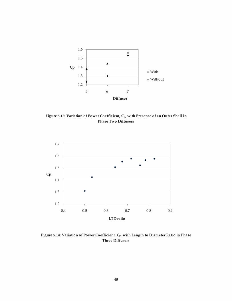
value of ring overlap was 0.92% of the rotor diameter. The addition of an

40

outer shell resulted in a decreased level of augmentation for the cases

examine in this phase, see Figure 5.13.

5.4. Final Design Optimizat ion Phase

5.4.1. LTDR Re-examined

Based on the CP versus EAR finding in the previous section a smaller 2.52

EAR diffuser was used to re-examine the LTDR relationship over a wider

range of values, see Table 5.3. This phase revealed a different

relationship. CP versus LTDR showed an asymptotic relationship. Once

fully attached flow was attained, roughly around a 0.7 LTDR, the

performance gains quickly leveled off, see Figure 5.14. The longer

diffusers also displayed a more narrow range of peak values similar to the

findings in the phase two study, see Figure 5.15. It is expected that as the

LTDR continued to increase there would be a reduction in augmentation

brought on by internal drag effects on the lengthy inner surface of the

diffuser. This may explain why some of Igra’s early designs with extreme

LTDRs performed more poorly than expected. The optimal LTDR most

certainly involves multiple variables including the EAR and additional

injected mass flow levels. It can be summed up, that as soon as an LTDR

is achieved that allows for minimal separation of flow for a given EAR

and supplemental mass flows, the returns of increased diffuser length

quickly diminish. In addition more length means more cost for

construction and more weight for support structure. The intention of this

41

phase of the study was to look at LTDR over a practical range to aid in the

later selection of design tradeoffs.

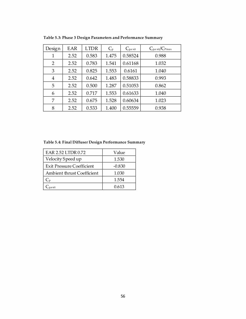
5.4.2. Final Diffuser Design

The final diffuser design had an EAR of 2.52 and a LTDR of 0.72. The

design exceeded the Betz limit by 4.0% based on the area of the diffuser

with a CP of 1.554 and CP,exit of 0.613, see Table 5.3. This figure was for a

rotor diameter of only 4.6m and a wind speed of just 5m/s. As discussed

in the study, with higher Reynolds number, comes more turbulent flow

reduced drag losses and higher values of power augmentation. Figure

5.16 shows the large sub-atmospheric pressure region in the wake of the

diffuser. The diffuser show a fairly wide peak performance region, see

Figure 5.17. It showed similar values of CP over a range of Ct from 0.30 to

0.45. When CP was plotted against Ct,amb the results showed a peak very

close to Ct,amb = 1, see Figure 5.18. This is the optimal Ct,amb value predicted

by Van Bussel [6]. An interesting finding is that the force exerted on the

diffuser by the wind is directly proportional to CP, see Figure 5.19. This

final diffuser also showed minimal signs of separation, see Figure 5.20.

5.5. Discussion

Exceeding the Betz limit based on EAR has been achieved in this CFD

study. However, the real world costs and compromises that the 1970’s

Grumman study focused on in great detail still exist [14]. These factors

include costs related to: diffuser material and construction, support

42

structure, and extreme wind loading. The fact that this study has

demonstrated the ability to exceed the Betz limit with an actual design

and detailed CFD analysis is a significant step in wind power research.

Up to this point only theoretical studies have shown that this task was

possible. The fact remains that the added structural requirements and

material costs associated the DAWT make it significantly more costly per

kWhr than a traditional wind turbine.

43

5.6. Figures

Figure 5.1: Variation of Power Coefficient, Cp, with Exit Angle in Phase One Diffusers

Figure 5.2: Variation of Power Coefficient, Cp, with Addition of Vortex Generator Tabs in Phase One Diffusers

0.60.70.80.9

11.11.2

22.5 30 45 Stepped 45

Cp

Angle

1

1.02

1.04

1.06

1.08

1.1

1.12

1.14

without with

Cp

44

Figure 5.3: Variation of Power Coefficient, Cp, with Presence of Gaps in Phase One Diffusers

Figure 5.4: Variation of Power Coefficient Cp, with the Presence of an Outer Skin in Phase One Diffusers

0.8

0.85

0.9

0.95

1

1.05

1.1

1.15

1.2

without with

Cp 30 Deg

Stepped

0.8

0.85

0.9

0.95

1

1.05

1.1

1.15

without with

Cp 30 Deg

Stepped

45

Figure 5.5: Variation of Power Coefficient, Cp, with Length to Diameter Ratio in Phase Two Diffusers

Figure 5.6: Variation of Power Coefficient, Cp, with Exit Area Ratio in Phase Two Diffusers

1.2

1.3

1.4

1.5

1.6

1.7

0.45 0.50 0.55 0.60 0.65 0.70

Cp

LTD

11.11.21.31.41.51.61.71.8

1.5 2 2.5 3 3.5

Cp

EAR

46

Figure 5.8: Variation of Power Coefficient, Cp, with Exit angle in Phase Two Diffusers

1.5

1.55

1.6

1.65

1.7

40 50 60

Cp,rotor

Exit angle

Figure 5.7: Variation of Specific Power Coefficient, Cp,exit, with Exit Area Ratio in Phase Two Diffusers

0.5

0.55

0.6

0.65

0.7

2 2.2 2.4 2.6 2.8 3

Cp,exit

EAR

47

Figure 5.9: Variation of Power Coefficient, Cp, with Wind speed in Phase Two Diffusers

Figure 5.10: Variation of Power Coefficient, Cp, with Inlet Diameter in Phase Two Diffusers

1.61.621.641.661.68

1.71.721.74

0 5 10 15 20

Cp

Wind Speed (m/s)

1.61.611.621.631.641.651.661.671.68

12.8 13 13.2 13.4

Cp

Inlet diameter

48

Figure 5.11: Variation of Power Coefficient, Cp, with Ring Gap Size in Phase Two Diffusers

Figure 5.12: Variation of Power Coefficient, Cp, with Ring Overlap Distance in Phase Two Diffusers

1.5

1.55

1.6

1.65

1.7

0.06 0.07 0.08 0.09 0.1 0.11

Cp

Ring Gap

1.5

1.55

1.6

1.65

1.7

0 0.1 0.2 0.3

Cp

Ring Overlap

49

Figure 5.13: Variation of Power Coefficient, Cp, with Presence of an Outer Shell in Phase Two Diffusers

Figure 5.14: Variation of Power Coefficient, Cp, with Length to Diameter Ratio in Phase Three Diffusers

1.2

1.3

1.4

1.5

1.6

5 6 7

Cp

Diffuser

With

Without

1.2

1.3

1.4

1.5

1.6

1.7

0.4 0.5 0.6 0.7 0.8 0.9

Cp

LTD ratio

50

Figure 5.15: Variation of Power Coefficient, Cp, with Local Thrust Coefficient in Phase Three Diffusers

1.100

1.150

1.200

1.250

1.300

1.350

1.400

1.450

1.500

1.550

1.600

0.3 0.4 0.5 0.6 0.7

Cp

Ct

0.83

0.78

0.72

0.68

0.64

0.58

0.53

0.5

51

Figure 5.16: Pressure Gradient of Final Diffuser Demonstrating a Sub-atmospheric Pressure in a Large Wake Zone

Figure 5.17: Variation of Power Coefficient with Local Thrust Coefficient for Final Diffuser Demonstrating a Peak Value Near 0.38.

1.20

1.25

1.30

1.35

1.40

1.45

1.50

1.55

1.60

0.2 0.3 0.4 0.5 0.6 0.7 0.8

Cp

Ct

52

Figure 5.18: Variation of Power Coefficient with Ambient Thrust Coefficient for Final Diffuser Demonstrating a Peak Value Near 1.0

1.530

1.535

1.540

1.545

1.550

1.555

1.560

0.90 0.95 1.00 1.05 1.10

Cp

Ct

53

Figure 5.19: Variation of Force with Local Thrust coefficient

Figure 5.20: Velocity Gradient of Final Diffuser Showing Minimal Signs of Separation at the Rear Edge of the Diffuser

420

430

440

450

460

470

480

490

0.2 0.3 0.4 0.5 0.6 0.7 0.8

Force (N)

Ct

54

5.7. Tables

Table 5.1: Phase 1 Design Parameters and Results

Run Cp Half Angle Vortex

Generators Slats Skins 1111 1.119 30 N N 1 1112 1.105 30 Y N 1 1121 1.089 30 N Y 1 1221 1.100 30 N Y 2 2111 1.191 22.5 N N 1 3111 0.772 45 N N 1 4111 1.071 50 stepped N N 1 4121 0.860 50 stepped N Y 1 4221 0.865 50 stepped N Y 2

55

Table 5.2: Phase 2 Design Parameters and Performance Summary

Profile Cp Ct at Peak Cp

EAR LTDR CP/CP,e xit

6 1.440 0.55 3.00 0.533 2.429 6.2 1.299 0.60 3.00 0.533 2.190 8 1.565 0.50 3.00 0.646 2.639

8.2 1.529 0.42 3.00 0.646 2.579 9 1.612 0.42 3.00 0.648 2.718 10 1.646 0.40 3.00 0.640 2.775 11 1.638 0.40 3.00 0.636 2.762 12 1.634 0.45 3.00 0.617 2.756 13 1.662 0.40 3.00 0.659 2.802

13.5 1.596 0.40 2.75 0.631 2.692 14 1.642 0.35 3.00 0.640 2.770 15 1.659 0.40 3.00 0.672 2.798 16 1.599 0.40 3.00 0.651 2.697 17 1.669 0.40 3.00 0.659 2.814

17.2 1.598 0.40 2.75 0.658 2.695 17.4 1.514 0.40 2.50 0.587 2.553 17.6 1.422 0.45 2.35 0.585 2.398 17.8 1.209 0.50 2.00 0.532 2.039 18 1.595 0.45 3.00 0.662 2.690 19 1.624 0.45 3.00 0.658 2.739 20 1.611 0.45 3.00 0.654 2.716 21 1.333 0.55 3.00 0.509 2.249

56

Table 5.3: Phase 3 Design Parameters and Performance Summary

Design EAR LTDR Cp Cp,e xit Cp,e xit/CPmax

1 2.52 0.583 1.475 0.58524 0.988 2 2.52 0.783 1.541 0.61168 1.032 3 2.52 0.825 1.553 0.6161 1.040 4 2.52 0.642 1.483 0.58833 0.993 5 2.52 0.500 1.287 0.51053 0.862 6 2.52 0.717 1.553 0.61633 1.040 7 2.52 0.675 1.528 0.60634 1.023 8 2.52 0.533 1.400 0.55559 0.938

Table 5.4: Final Diffuser Design Performance Summary

EAR 2.52 LTDR 0.72 Value Velocity Speed up 1.530 Exit Pressure Coefficient -0.830 Ambient thrust Coefficient 1.030 Cp 1.554 Cp,exit 0.613

57

CHAPTER 6: CONCLUSION

The increase in computing power and the proliferation of CFD software

has made it possible to reassess the work of previous researchers without

the massive funding that was necessary to fund the original studies. The

days of going straight from the drawing board to a test lab are long gone.

The idea of augmenting wind power collection devices has been around

since wind power collection itself. The diffuser augmented wind turbine

in its present sense has been developed over the last 50 years. During this

time there have been numerous studies funded by governments and large

companies. Most of these studies made an effort to understand important

geometry parameters and there effects on power augmentation. Studies

like those conducted by Grumman and Auckland made compromises for

cost effectiveness too early in their work to fully explore the limits of the

diffuser augmented wind turbine. By initially restricting the diffuser

LTDR they effectively put a limit on how efficient the diffusers they test

could be.

This thesis set out to find if, as momentum theory predicts, the diffuser

augmented wind turbine can exceed the Betz limit based on its exit area.

To that question the answer has been presented; yes. The final diffuser

design had an EAR of 2.52 and a LTDR of 0.72. The final design that was

analyzed in this study exceeded the Betz limit by 4.0% based on the area

of the diffuser with a Cp of 1.554 and a CP,Betz of 2.62. This figure was for a

58

rotor diameter of only 4.6m and a wind speed of 5m/s. As discussed in

the study, with higher Reynolds number, comes more turbulent flow,

reduced drag losses, and higher values of Cp. The figures in this study are

based on area averaged velocity and pressure outputs which proved to be

more conservative and consistent than the pressure and velocity readings

taken at diffuser mounted pressure ports and single point anemometers.

This study did also not include rotor tip vortex generation or wake

rotation and the beneficial effects they had on separation delay in the

boundary layer and resulting increased augmentation [22]. When testing

with a rotor in place it is expected that the available power based on

pressure readings will be higher than the CFD results because of these

phenomena.

6.1. Recommended Future Studies

The next step for this design is to verify the findings of this thesis with

wind tunnel testing. For a comparison with results in the CFD study,

initial testing should be performed with the wind turbine simulated by a

filter or mesh with resistance equal to the optimal Ct. The wind tunnel

testing would need to replicate the Reynolds numbers seen in this study

for a valid comparison. This could be performed using a pressurized

wind tunnel, or more likely, higher wind velocity. Assuming the findings

of such testing verify the results presented in this thesis, a rotor would be

designed for the thrust coefficient and velocity profile of the final diffuser

design.

59

A model should be chosen to provide a thrust coefficient near the peak

efficiency of the diffuser, in the 0.35 to 0.45 range. This would be followed

by wind tunnel testing. At this point it would be expected that the

beneficial results of blade tip vortices on improving the potential for

energy capture would result in a higher Cp than found in this study. Up to

this point the Cp was based on pressure and velocity readings. Once the

power is defined by a torque and rotational speed, instead, losses

associated with a particular blade design will become a major factor in the

performance of the system.

60

REFERENCES

[1] Global Wind Energy Council (GW EC). GWEC Global Wind 2009 Report. [Report on the Internet]. Belgium: GWEC; 2010 [cited 2010 June 13]. [66 p]. Available from: http://www.gwec.net/fileadmin/documents/Publications/Global_Wind_2007_reprep/GWEC_Global_Wind_2009_Report_LOWRES_15th.%20Apr..pdf.

[2] Singer C, Holyward EJ, Hall AR, Williams TI. A History of Technology, Volume II: The Mediterranean Civilizations and the Middle Ages. Oxford: Clarendon Press; 1956. 846 p.

[3] Sathyajith M. Wind Energy: Fundamentals, Resource, Analysis and Economics.

Netherlands: Springer; 2006. 246 p.

[4] Veers PS, Butterfield S. Extreme Load Estimation for Wind Turbines: Issues and Opportunities for Improved Practice. 2001 ASME Wind Energy Symposium. Reno, Nevada, AIAA-2001-0044; 2001. 10 p. Available from: http://windpower.sandia.gov/asme/aiaa-2001-004.pdf

[5] Burton T, Sharpe D, Jenkins N, Bossanyi E. Wind Energy Handbook. England:

John Wiley & Sons, Ltd; 2001. 642 p.

[6] Van Bussel GJW. The Science of Making More Torque From Wind: Diffuser Experiments and Theory Revisited. Journal of Physics: Conference Series, IOP Publishing 2007;75:1-12. Available from: http://iopscience.iop.org/1742-

6596/75/1/012010.

[7] Jamieson PM. Beating Betz: Energy Extraction Limits in a Constrained Flow

Field. Journal of Solar Energy Engineering 2009;131(3). 6 p.

[8] Jamieson P. Generalized Limits for Energy Extraction in a Linear Constant Velocity Flow Field. Wind Energy 2008; 11:445–457.

61

[9] Phillips DG. An Investigation on Diffuser Augmented Wind Turbine Design [PhD Dissertation]. New Zealand: Auckland University; 2003 [cited 2010 June 18]. [334 p]. Available from: http://researchspace.auckland.ac.nz/handle/2292/1940.

[10] American Wind Energy Association (AWEA). The US Small Wind Turbine Industry, Roadmap, A 20-Year Industry Plan for Small Wind Turbine Technology. Golden, Colorado: National Wind Energy Center; 2002 [Cited 2010 June 12]. [47 p]. Available from: http://www.awea.org/smallwind/documents/31958.pdf

[11] Foreman KM. Size Effects in DAWT Innovative Wind Energy System Design.

Solar Energy Engineering 1983;105: 401-407.

[12] Foreman KM. Diffuser Augmented Wind Turbine. Solar Energy 1978; 20:305-

311.

[13] Gilbert BL, Foreman KM, Experiments with a Diffuser-Augmented Model Wind Turbine. Journal of Energy Resources Technology 1983;105:46-53.

14] Foreman KM. Preliminary Design and Economic Investigations of Diffuser Augmented Wind Turbines (DAWT). Golden, Colorado: Solar Energy Research Institute; 1981[cited 2010 May 22]. [36 p]. Available from: http://www.nrel.gov/docs/legosti/old/98073-1A.pdf.

[15] Igra O. Research and Development for Shrouded Wind Turbines. Energy

Conversion and Management 1981;21:13-48.

[16] Bet F, Grassmann H. Upgrading Conventional Wind Turbines. Renewable

Energy 2003;28:71–78.

62

[17] Tokuyama H, Ushiyama I, Seki K. Experimental Determination of Optimum Design Configuration for Micro Wind Turbines at Low Wind Speeds. Wind Engineering 2002;26(1):39-49.

[18] Hansen MOL, Sorensen NN, Flay RGJ. Effect of Placing a Diffuser Around a Wind Turbine. Wind Energy John Wiley & Sons, Ltd. 1999;3:207–213.

[19] Abe K, Nishida M, Sakurai A, Ohya Y, Kihara H, Wada E, Sato K. Experimental and Numerical Investigations of Flow Fields Behind a Small Wind Turbine with a Flanged Diffuser. Journal of Wind Engineering and Industrial Aerodynamics 2005; 93:951–970.

[20] Velte CM, Hansen MOL, Jonck K. Experimental and Numerical Investigation of the Performance of Vortex Generators on Separation Control. Journal of Physics: Conference Series. IOP Publishing 2007[cited 2010 June 4];75:[11 p]. Available from: http://iopscience.iop.org/1742-6596/75/1/012030.

[21] Logdberg O, Angele K, Alfredsson PH. On the Robustness of Separation Control

by Streamwise Vortices. European Journal of Mechanics B/Fluids 2010;29:9-17.

[22] Fletcher CAJ. Computational Analysis of Diffuser-Augmented Wind Turbines. Energy Conversion and Management 1981; 21:175-183.

[23] Leschziner MA. Modelling Turbulent Sseparated Flow in the Context of

Aerodynamic Applications. Fluid Dynamics Research 2006; 38:174–210.

[24] Torresi M, Camporeale SM, Strippoli PD, Pascazio G. Accurate Numerical Simulation of a High Solidity Wells Turbine. Renewable Energy 2008;33: 735–747.

63

APPENDIX A: TURBULENCE MODEL COMPARISON

The STAR CCM+ Spalart-Allmaras, S-A, Turbulence solver was used to

compare to the results of the K-ε turbulence analysis’. The K-ε model is a

robust model in a wide variety of flow applications and was chosen for

the primary solver for this study due to the author’s familiarity and

comfort level with it. The S-A Turbulence model is recommended for

aerodynamic flows around curved shapes such as turbine blades and

airfoils [23]. It is also known as well suited for primarily attached flows in

which separation effects are minimal [24].

The S-A Turbulence model showed minor improvements in Cp as

compared to the K-ε model. The peak value of Cp for the S-A model was

1.568 compared to the peak value of 1.553 for the K-ε model, see Figure

B.1. This is a difference of only 0.9% at the highest Cp values. The most

noticeable differences occurred at non-optimum Ct values. For these non-

optimum cases the S-A model predicted a Cp up to 8.7 % higher than the K-

ε model. This can be explained by the different methods that these two

models predict separation of flow and the S-A model’s intended use for

largely attached flows [23]. For the purposes of this study in which the

peak Cp values are the values of interest, the K-ε turbulence model

compares very closely with the more specialized S-A model. In addition it

provides a more conservative estimate of Cp based on its earlier prediction

of separated flow and appears to be a valid choice.

64

A.1 F igures

Figure A.1: Comparison of Power coefficient, Cp, versus Thrust Coefficient, Ct, using K-Epsilon and Spalart-Allmaras Turbulence Models

1.200

1.300

1.400

1.500

1.600

1.700

1.800

0.2 0.3 0.4 0.5 0.6 0.7 0.8

Cp

Ct

S-A

K-E

65

APPENDIX B: COMPARISON TO PREVIOUS TESTS

One of the most important elements of an analytical study is correlation

back to empirical results or theory. In this study three separate cases were

analyzed and compared back to results from previous tests and theory.

The first of these comparative studies was a bare turbine. A bare turbine

was simulated using the same filter element that was used in the various

diffuser studies. The only difference was the lack of a diffuser. The

second case was a simulation examining the Grumman study diffuser

with a 2.78 EAR and LTDR of 0.715. The third case looked a diffuser from

the Auckland study. This diffuser had an EAR of 3.0 and a LTDR of 0.488.

All of the cases used the same test setup as the other phases of this study.

The details of this test setup can be found in Chapter 4.

B.1 Bare Turbine

The first case looked at a bare rotor. The bare rotor was simulated using a

filter modeled as a porous media. The thrust coefficient of this filter was

varied. Area averaged velocity at the upstream plane of the filter. Area-

averaged pressures were recorded for the upstream and downstream

planes of the filter to give a pressure difference across the rotor. Plugging

these measurements into Equation 4.1 yielded a power coefficient. The

resulting power coefficients at various thrust coefficients were recorded

for the filter element representation of a rotor. These results were then

compared back to the theoretical relationship.

66

(B.1)

The results of this comparison were plotted in Figure B.1. The difference

between the theoretical values based on actuator disc theory and the Cp

values based on area averaged velocity and pressure difference was less

than 1.7% for all values of Ct.

B.2 Grumman Diffuser

The second case examined the Grumman DAWT. This was modeled at

the same scale as the actual test, see Figure B.2. The Diffuser model was

created based on figures from the Grumman paper [13]. The rotor

diameter was 0.46m and the wind tunnel velocity was 36 m/s, see Figure

B.3. There have been some questions about the validity of the power

coefficients that were published in the Grumman paper [9]. Upstream

pressure readings were taken on leading edge of the diffuser. This would

yield a higher pressure than that seen at the leading plane of a rotor and

would thus give the impression of a greater than actual power coefficient.

The peak Cp value in this CFD study was 1.12 at a Ct of 0.95. As presented

in the Grumman paper this value of Cp would be divided by the Betz limit

to yield an Augmentation level of 1.89. The results of the study are

plotted in Figure B.4. Grumman estimated an Augmentation level of 2.75.

Phillips evaluated the same Grumman diffuser and estimated an

Augmentation level of 1.85 [9]. This correlates closely with value found in

this CFD study, with a difference of only 2.1%.

67

B.3 Auckland Diffuser

The third case looked at the diffuser developed in the Auckland study, see

Figure B.5. This study used a 0.48 m diameter diffuser with a wind tunnel

velocity of 10.5 m/s, see Figure B.6. The peak Cp value in this CFD study

was 1.12 at a Ct,∞ of 0.98. As presented in the Auckland paper this value of

Cp would be divided by the Betz limit to yield a peak augmentation level

of 1.88. The results of the study are plotted in Figure B.7. Phillips

estimated an Augmentation level of 1.73 based on pressure and velocity

readings [9]. In this case, the CFD results yielded a higher augmentation,

with a difference of 8.7%. This slightly exaggerated performance is not a

cause for concern given the lack of design details available for the

Auckland Diffuser. The CFD study used a diffuser design that was

modeled to represent the Auckland design based on solely on

incompletely dimensioned diagrams.

68

B.4 Figures

Figure B.1: Comparison of Theoretical and Analytical Models of a Bare Wind Turbine

Figure B.2: Author’s interpretation of Grumman Diffuser

0.000

0.100

0.200

0.300

0.400

0.500

0.600

0.700

0.000 0.200 0.400 0.600 0.800 1.000

Cp

Ct

Cp

Actuator Disc Theory

69

Figure B.3: Velocity Gradient Plot of Grumman Diffuser Showing Large Area of Separated Flow

Figure B.4: CFD Results for Variation of Power Coefficient with Thrust Coefficient for Grumman Diffuser Design

0.800

0.900

1.000

1.100

1.200

0.3 0.5 0.7 0.9 1.1

Cp

Ct

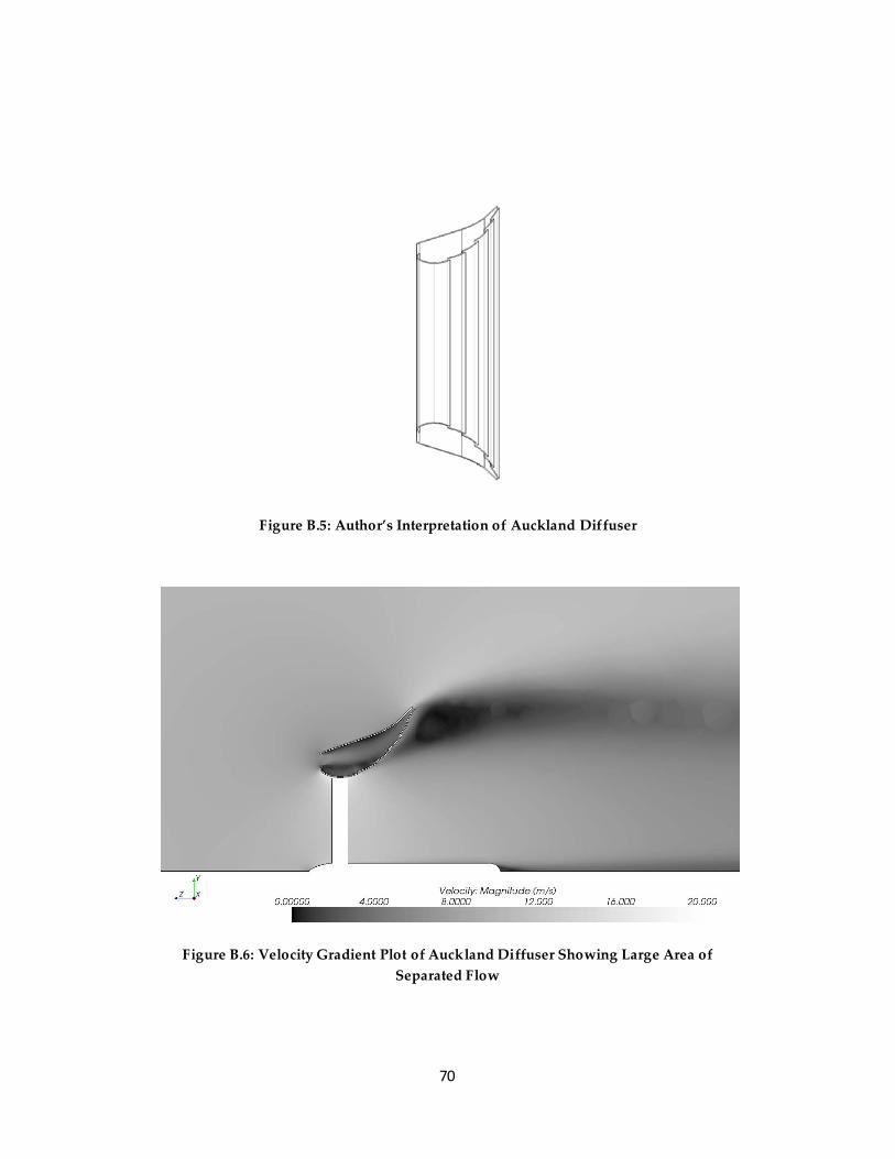
70

Figure B.5: Author’s Interpretation of Auckland Diffuser

Figure B.6: Velocity Gradient Plot of Auckland Diffuser Showing Large Area of Separated Flow

71

Figure B.7: CFD Results of Variation of Power Coefficient with Local Thrust Coefficient for Auckland Design

1.70

1.72

1.74

1.76

1.78

1.80

1.82

1.84

1.86

1.88

1.90

0.40 0.60 0.80 1.00 1.20 1.40

Cp

Ct

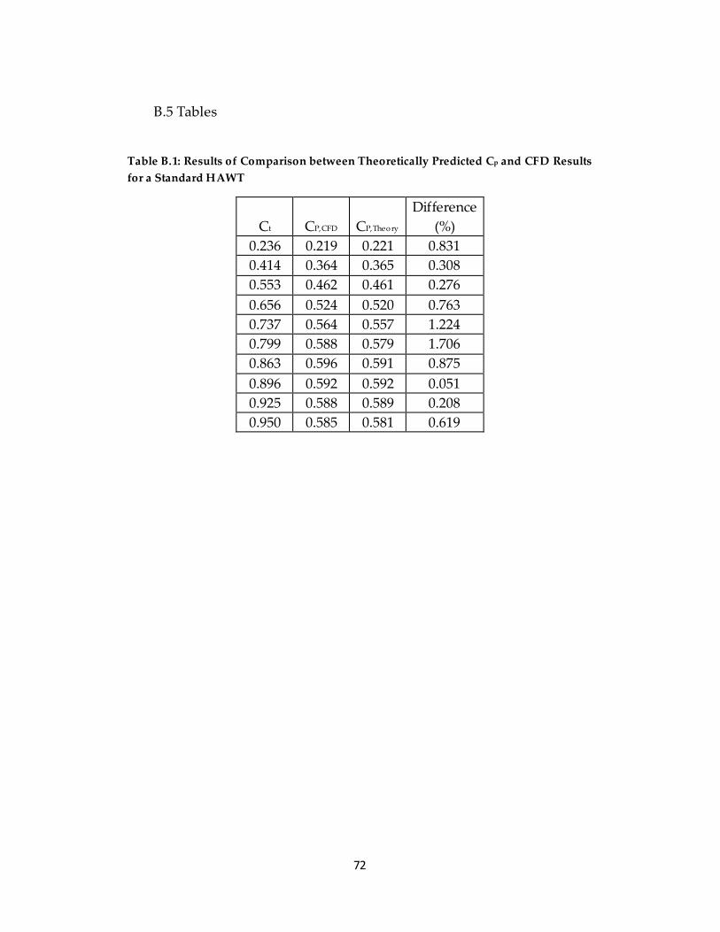
72

B.5 Tables

Table B.1: Results of Comparison between Theoretically Predicted Cp and CFD Results for a Standard HAWT

Ct CP,CFD CP,Theory Difference

(%) 0.236 0.219 0.221 0.831 0.414 0.364 0.365 0.308 0.553 0.462 0.461 0.276 0.656 0.524 0.520 0.763 0.737 0.564 0.557 1.224 0.799 0.588 0.579 1.706 0.863 0.596 0.591 0.875 0.896 0.592 0.592 0.051 0.925 0.588 0.589 0.208 0.950 0.585 0.581 0.619