Elad Alon, BabakAyazifar, GireejaRanade, Vivek Subramanian ...
date post
19-Dec-2015Category
view
214download
0
- 1 -
Fast Polar Fourier Transform
Michael Elad*Scientific Computing and Computational Mathematics
Stanford University
FoCM Conference, August 2002
Image and Signal Processing Workshop
IMA - Minneapolis
* Joint work with Dave Donoho (Stanford-Statistics), Amir Averbuch (TAU-CS-Israel), and Ronald Coifman (Yale-Math)

- 2 -
Collaborators
Dave DonohoStatistics
Department Stanford
Amir AverbuchCS Department Tel-Aviv University
Ronald Coifman
Math. Department Yale
- 3 -
Fast Polar Fourier Transform
FFT is one of top 10 algorithms of 20th
century.
We'll extend utility of FFT algorithms to new
class of settings in image processing.
Create a tool which is: Free of emotional involvement, &
Freely available over the internet.
Current Stage: We have the tool, and its analysis,
Have not demonstrated applications yet.
- 4 -
Agenda
1. Thinking Polar – Continuum
2. Thinking Polar – Discrete
3. Current State-Of-The-Art
4. Our Approach - General
5. The Pseudo-Polar Fast Transform
6. From Pseudo-Polar to Polar
7. Algorithm Analysis
8. Conclusions
Thinking Polar – Continuum Background &
Motivation
New Approach
and its Results

- 5 -
1. Thinking Polar - Continuum
For today f(x,y) function of (x,y)2
Continuous Fourier Transform
dxdyiyvixuexpy,xfy,xfv,uf̂
dxdy)sin(iy)cos(ixrexpy,xf
)sin(r),cos(rf̂,rf~
Polar coordinates: u=r·cos() , v=r·sin()
Important Processes easy to continuum polar
domain.

- 6 -
-5 -4 -3 -2 -1 0 1 2 3 4 5
-5
-4
-3
-2
-1
0
1
2
3
4
5
v
u
0 1 2 3 4 5 6 7
0
1
2
3
4
5
6
r
1. Thinking Polar - Continuum
r

- 7 -
Natural Operations: 1. Rotation
Using the polar coordinates, rotation is simply a
shift in the angular variable.
1. Thinking Polar - Continuum
Q0 – planar rotation by 0 degrees
Rotation
In polar coordinates – shift in angular variable
y,xQfy,xf00
0,rf~
,rf~
0

- 8 -
Natural Operations: 2. Scaling
Using the polar coordinates, 2D scaling is simply a
1D scaling in the radial variable.
1. Thinking Polar - Continuum
S – planar scaling by a factor
Scaling
In polar coordinates – 1D scale in radial variable
Log-Polar – shift in the radial variable.
y,xSfy,xf
,rf~
Const,rf~

- 9 -
Natural Operations: 3. Registration
Using the polar coordinates, rotation+shift
registration simply amounts to correlations.
1. Thinking Polar - Continuum
f(x,y) and g(x,y):
Goal: recover .
Angular cross-correlation between
– Estimate 0.
Rotation & cross-correlation on regular Fourier
transform gives the shift.
00 y,xy,xQgy,xf0
000 ,y,x
,rg~and,rf~
- 10 -
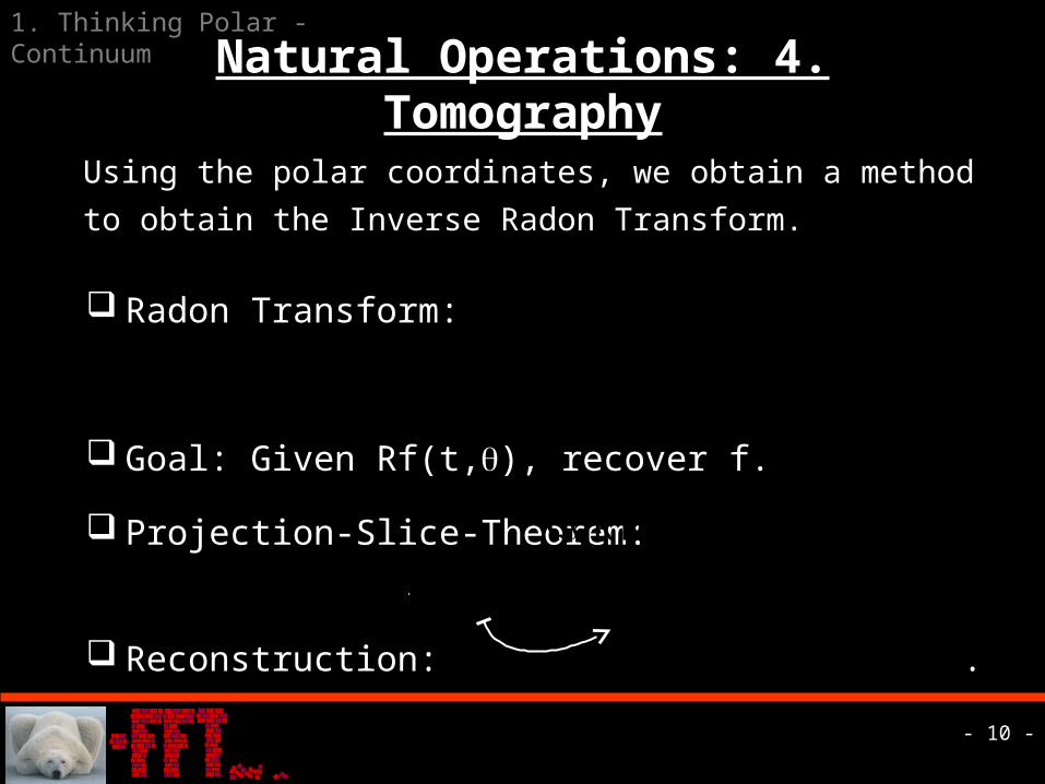
Natural Operations: 4. Tomography
Using the polar coordinates, we obtain a method
to obtain the Inverse Radon Transform.
1. Thinking Polar - Continuum
Radon Transform:
Goal: Given Rf(t,), recover f.
Projection-Slice-Theorem: .
Reconstruction: .
dxdyt)sin(y)cos(x)y,x(f,tRf
,rf~
,tRf1
ff̂f~
Rf

- 11 -
More Natural Operations
1. Thinking Polar - Continuum
New orthonormal bases:
Ridgelets,
Curvelets,
Fourier Integral operations,
Ridgelet packets.
Analysis of textures.
Analysis of singularities.
More …
r
- 12 -
Agenda
1. Thinking Polar – Continuum
2. Thinking Polar – Discrete
3. Current State-Of-The-Art
4. Our Approach - General
5. The Pseudo-Polar Fast Transform
6. From Pseudo-Polar to Polar
7. Algorithm Analysis
8. Conclusions

- 13 -
2. Thinking Polar - Discrete
Certain procedures very important to digitize Rotation,
Scaling,
Registration,
Tomography, and
…
These look so easy in continuous theory –
Can’t we use it in the discrete domain?
Why not Polar-FFT?

- 14 -
The FFT Miracles
1D Discrete Fourier Transform
Uniformly sampled in time and frequency –
FFT.
Complexity – O(5Nlog2N) instead of O(N2).
2. Thinking Polar - Discrete
2D Discrete Fourier Transform
Cartesian grid in space and frequency – Separability
Only 1D-FFT operations.
Smart memory management.

- 15 -
2D DFT – Cartesian Grid
2. Thinking Polar - Discrete
N2
N21
2N
2N
n,n2y
1x
21Nn2
Nn2
-
-
x
y

- 16 -
1D FFT to rows5N2logN
Cartesian 2D-FFT
10N2logN
Cartesian Data
N-by-N
1D FFT to columns
5N2logN
2D FFT Complexity
Complexity:
O(10N2log2N) instead
of O(N4).
Important Feature: All
operations are 1D
– leading to
efficient cache
usage

- 17 -
Discrete Polar Coordinates?
2. Thinking Polar - Discrete
Choice of grid?
-
-
,NSn
r1NS
0nr
1r
1
rNS
Resulting with NS
rays with NSr
elements on each:
For S=Sr=1, we
have N2 grid points.
NS2
1NS
0n
2
2NS
n2
x
y

- 18 -
Grid Problematics
2. Thinking Polar - Discrete
Grid spacing?
Fate of corners?
No X-Y separability !!
-
-
x
y

- 19 -
Polar FFT - Current Status
2. Thinking Polar - Discrete
Current widespread belief - There cannot be
a fast method for DFT on the polar grid. See
e.g. The DFT: an owner’s manual, Briggs
and Henson, SIAM, 1995, p. 284.
Consequence of Non-existence: Continuous Fourier – vague inspiration only.
Fourier in implementations widely deprecated.
Fragmentation: each field special algorithm.

- 20 -
Agenda
1. Thinking Polar – Continuum
2. Thinking Polar – Discrete
3. Current State-Of-The-Art
4. Our Approach - General
5. The Pseudo-Polar Fast Transform
6. From Pseudo-Polar to Polar
7. Algorithm Analysis
8. Conclusions

- 21 -
3. Current State-Of-The-Art
Assessing T: Unequally-spaced FFT (USFFT)
Data in Cartesian set.
Approximate transform in non-Cartesian
set.
Oriented to 1D – not 2D and definitely not
Polar. Assessing T
†: For Tomography
Data in Polar coordinates in frequency.
Approximate inverse transform to
Cartesian grid.
Inspired by the projection-slice-theorem.

- 22 -
USFFT - Rational
3. Current State-of-the-Art
-3 -2 -1 0 1 2 3
-3
-2
-1
0
1
2
3
+ Destination Polar grid
O Critically sampled Cartesian grid
o Over-sampled Cartesian grid
x
y

- 23 -
USFFT - Detailed
Over-sample Cartesian grid.
Rapidly evaluate FT:
Values F.
Possibly - partial derivatives.
Associate Cartesian neighbors to each
polar grid point.
Approximate interpolation.
3. Current State-of-the-Art

- 24 -
Our Reading of Literature
3. Current State-of-the-Art
Boyd (1992) – Over-sampling and
interpolation by Euler sum or Langrangian
interpolation.
Dutt-Rokhlin (1993,1995) - Over-sampling
and interpolation by the Fast-Multipole
method.
Anderson-Dahleh (1996) – Over-sampling and
obtaining the partial derivatives, and then
interpolating by Taylor series.
Ware (1998) – Survey on USFFT methods.

- 25 -
USFFT Problematics
3. Current State-of-the-Art
Several involved parameters:
Over-sampling factor,
Method of interpolation, and
Order of interpolation.
Good accuracy calls for extensive over-sampling.
Correspondence overhead: spoils vectorizability of algorithm - causes high cache misses.
Emotionally involved.

- 26 -
Agenda
1. Thinking Polar – Continuum
2. Thinking Polar – Discrete
3. Current State-Of-The-Art
4. Our Approach - General
5. The Pseudo-Polar Fast Transform
6. From Pseudo-Polar to Polar
7. Algorithm Analysis
8. Conclusions

- 27 -
4. Our Approach - General
Low complexity – O(Const·N2log2N)
Vectorizability – 1D operations only
Non-Expansiveness – Factor 2 (or 4) only
Stability – via Regularization
Accuracy – 2 orders of magnitude over USFFT
methods
We propose a
Fast Polar Fourier Transform
with the following features:

- 28 -
Our Strategy
Fast and Exact Fourier Trans. on a polar-like
grid
1D interpolation
s to the polar grid
Pseudo Polar Grid
- 29 -
Agenda
1. Thinking Polar – Continuum
2. Thinking Polar – Discrete
3. Current State-Of-The-Art
4. Our Approach - General
5. The Pseudo-Polar Fast Transform
6. From Pseudo-Polar to Polar
7. Algorithm Analysis
8. Conclusions

- 30 -
5. The Pseudo-Polar FFT
Developed by Averbuch, Coifman,
Donoho, Israeli, and Waldén (1998).
Basic idea: A “Polar-Like” grid that enables
EXACT Fourier transform,
FAST computation,
1D operations only.
Applications: Tomography, image
processing, Ridgelets, and more.
- 31 -
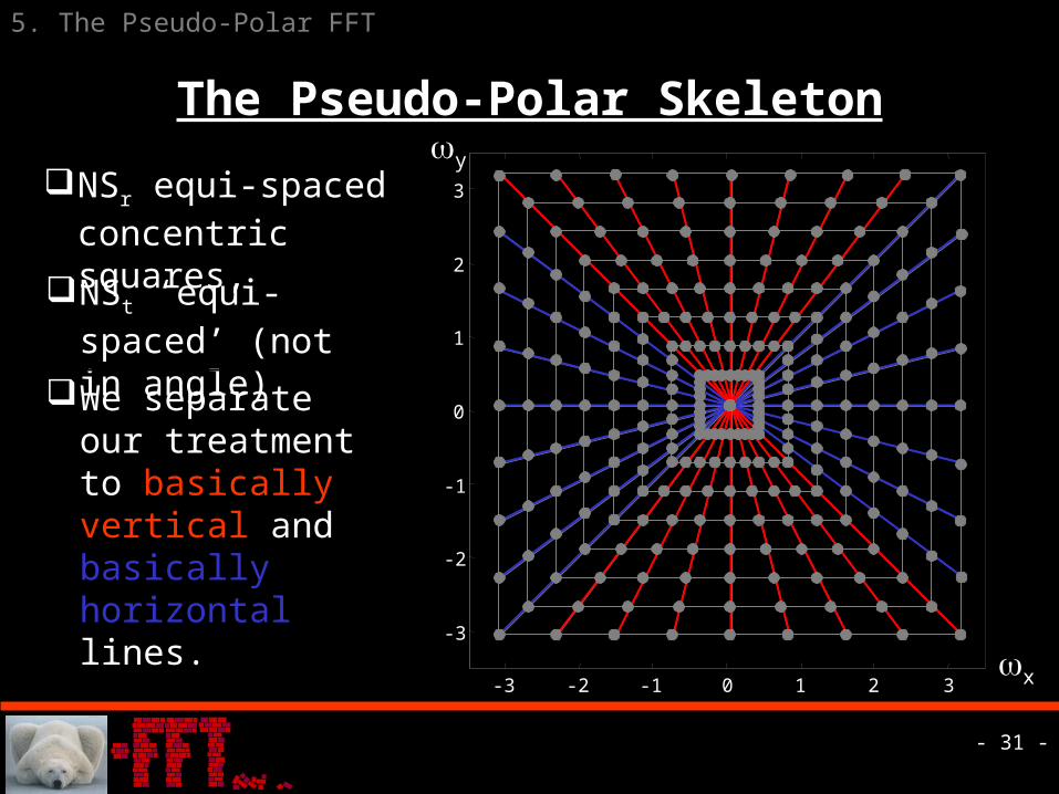
The Pseudo-Polar Skeleton
5. The Pseudo-Polar FFT
-3 -2 -1 0 1 2 3
-3
-2
-1
0
1
2
3
x
yNSr equi-spaced
concentric squares,NSt ‘equi-spaced’ (not in angle)
We separate our treatment to basically vertical and basically horizontal lines.
- 32 -
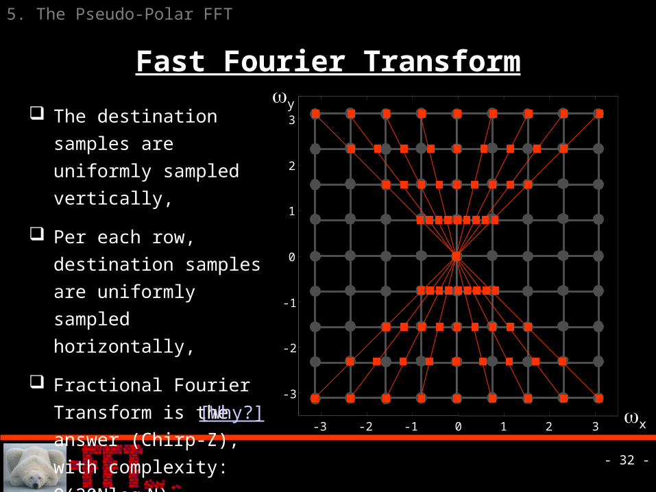
Fast Fourier Transform
5. The Pseudo-Polar FFT
x
y
-3 -2 -1 0 1 2 3
-3
-2
-1
0
1
2
3 The destination
samples are uniformly
sampled vertically,
Per each row,
destination samples
are uniformly sampled
horizontally,
Fractional Fourier
Transform is the
answer (Chirp-Z), with
complexity:
O(20Nlog2N).
[Why?]

- 33 -
PP-FFT versus 2D-FFT
5. The Pseudo-Polar FFT
1D FFT to columns
5N2logN
1D FFT to rows5N2logN
Cartesian 2D-FFT
10N2logN
1D FFT to columns
5N2logN
1D FRFFT to rows20N2logN
PP-FFT vertical25N2log
N
Cartesian Data
N-by-N
2D-FFTPP-FFT

- 34 -
The PP-FFT - Properties
5. The Pseudo-Polar FFT
Exact in exact arithmetic.
No parameters involved !!
Complexity - O(50·N2log2N) versus
O(N4).
1D operations only.
For the chosen grid (Sr=St=2) - 5.

- 35 -
Agenda
1. Thinking Polar – Continuum
2. Thinking Polar – Discrete
3. Current State-Of-The-Art
4. Our Approach - General
5. The Pseudo-Polar Fast Transform
6. From Pseudo-Polar to Polar
7. Algorithm Analysis
8. Conclusions

- 36 -
6. From Pseudo-Polar to Polar
Fast and Exact Fourier Trans. on a polar-like
grid
2 stages of 1D
interpolations to get to the polar
grid

- 37 -
The Interpolation Stages
6. From Pseudo-Polar to Polar
-3 -2 -1 0 1 2 3
-3
-2
-1
0
1
2
3
The original Pseudo-Polar Grid
Warping to equi-spaced angles
Warping each ray to have the same step
x
y

- 38 -
First Interpolation Stage
6. From Pseudo-Polar to Polar
-3 -2 -1 0 1 2 3
-3
-2
-1
0
1
2
3
Every row is a
trigonometric
polynomial of order N,
FRFT on over-sampled
array and 1D
interpolation,
Very accurate.
Rotation of the rays to have equi-spaced angles (S-Pseudo-Polar grid):
x
y
- 39 -
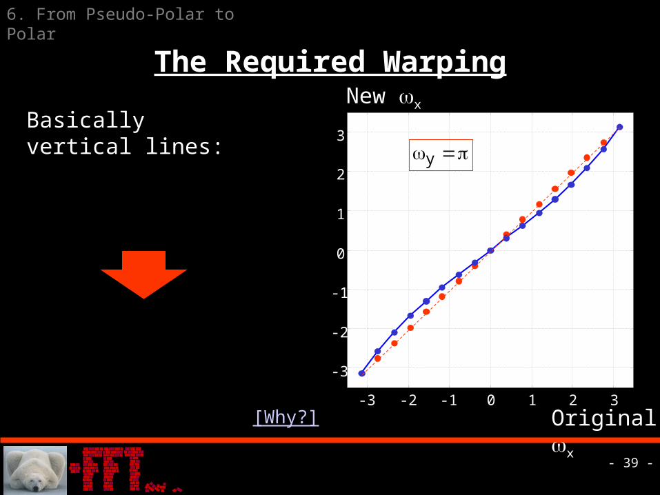
The Required Warping
6. From Pseudo-Polar to Polar
Basically vertical lines:
12NS
2NSm,
yt
xr
y
t
tNSm2
,NS2
12NS
2NSmt
yx
t
tNS2m
tan
-3 -2 -1 0 1 2 3
-3
-2
-1
0
1
2
3y
Original x
New x
[Why?]

- 40 -
The Actual Interpolation
6. From Pseudo-Polar to Polar
1D FFT to columns
5N2logN
1D FRFFT to rows
20N2logN
PP-FFT Vertical
25N2logN
Cartesian Data
N-by-N
S-PP-FFTPP-FFT
1D FFT to columns
5N2logN
1D Over-sampled (S) FRFFT to rows
20N2S·log(NS)
1D Interpolation
O{N2}
S-PP-FFT Vertical
(20S+5)N2logN

- 41 -
6. From Pseudo-Polar to Polar
Second Interpolation Stage
-3 -2 -1 0 1 2 3
-3
-2
-1
0
1
2
3
x
y
As opposed to the
previous step, the rays
are not trigonometric
polynomials of order N,
We proved that the rays
are band-limited
(smooth) functions,
Over-sampling and
interpolation is
expected to perform
well.

- 42 -
6. From Pseudo-Polar to Polar
Over-Sampling Along Rays
-3 -2 -1 0 1 2 3
-3
-2
-1
0
1
2
3 Over-sampling along rays cannot be done by taking the 1D ray and over-sampling it. Sr>1:
More concentric squares.
Sr longer 1D-FFT’s at the beginning of the algorithm.
Sr times FRFFT operations.
x
y

- 43 -
The Actual Interpolation
6. From Pseudo-Polar to Polar
Cartesian Data
N-by-N
1DFFT to over-sampled columns
N·5(NSr)·log(NSr
)
NSr·20(NSt)·log(NS
t) 1D Over-sampled (S) FRFFT to rows
1D Interpolation
O{(NSr)·N} O{N·N}
1D Interpolation
Polar-FFT Vertical
Full Polar FFT O{40SrStN2logN
}
S-PP-FFT Vertical
- 44 -
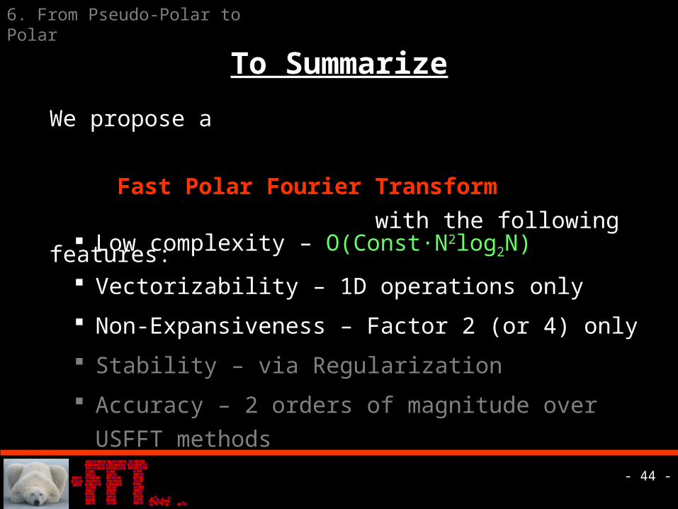
Low complexity – O(Const·N2log2N)
Vectorizability – 1D operations only
Non-Expansiveness – Factor 2 (or 4) only
Stability – via Regularization
Accuracy – 2 orders of magnitude over USFFT
methods
We propose a
Fast Polar Fourier Transform
with the following features:
To Summarize
6. From Pseudo-Polar to Polar

- 45 -
Agenda
1. Thinking Polar – Continuum
2. Thinking Polar – Discrete
3. Current State-Of-The-Art
4. Our Approach - General
5. The Pseudo-Polar Fast Transform
6. From Pseudo-Polar to Polar
7. Algorithm Analysis
8. Conclusions

- 46 -
7. Algorithm Analysis
We have a code performing the Polar-FFT in Matlab:
Where: X – Input array of N-by-N samples
St,Sr – Over-sampling factors in the approximations
Y – Polar-FFT result as an 2N-by-2N array with rows
being the rays and columns being the
concentric circles.
Y=Polar_FFT(X);
OR
Y=Polar_FFT(X,St,Sr);

- 47 -
The Implementation
7. Algorithm Analysis
The current Polar-FFT code implements
Taylor method for the first interpolation stage
and spline ONLY (no-derivatives) for the
second stage.
For comparison, we demonstrate the
performance of the USFFT method with over-
sampling S and interpolation based on the
Taylor interpolation (found to be the best).

- 48 -
10 20 30 40 50 60 70 80 90 100
10-3
10-2
10-1
100
101
102
St·Sr or S2
||Approximation error||1
Error for Specific Signal
7. Algorithm Analysis
Taylor USFFT
St=4
• Input is random 32-by-32 array,
• USFFT method uses one parameter whereas there are two for the up-sampling in the Polar-FFT.
• Thumb rule: Sr·St= S2.
St=2
St=3
St=1
Thumb rule: Sr=4St

- 49 -
Error For Specific Signals
7. Algorithm Analysis
Similar curves obtained of ||*|| and ||*||2 norms.
Similar behavior is found for other signals.
Conclusion: For the proper choice of St and Sr, we
get 2-orders-of-magnitude improvement in the
accuracy comparing to the best USFFT method.
Further improvement should be achieved for
Taylor interpolation in the second stage.
US-FFT takes longer due the 2D operations.

- 50 -
The Transform as a Matrix
7. Algorithm Analysis
All the involved
transformations (accurate
and approximate) are
linear - they can be
represented as a matrix
of size 4N2-by-N2.
Ya=AxOr
Yt=Tx
Approximate
True

- 51 -
Regularization of T/A
7. Algorithm Analysis
An input signal of N-by-N is transformed to an array or 2N-by-2N.
For N=16, T size is 1024-by-256, and 60,000 (bad for inversion).
0
yxxy
Corner
PolarPolar T
TT
Adding the assumption that the Frequency corners should be zeroed, we obtain
and the condition number becomes 5 !!!

- 52 -
Discarding the Corners?
7. Algorithm Analysis
-
-
2
2
2
2
If the given signal was sampled at 1.4142 the Nyquist Rate, the corners can be removed.
If it is not, over-sampling it can be done by FFT.

- 53 -
7. Algorithm Analysis
Error Analysis – Worst Signal
FFTPolarFFTPolar ex TAApproximation error is :
22
22
x x
xMax/Arge,x
PolarFFTPolar2worstworst
TA Worst error :
22
22
x x
xMax/Arge,x
Polar
PolarFFTPolar2rworstrworst
T
TA Worst relative error :

- 54 -
7. Algorithm Analysis
Worst Signal - Results
N=16 TC 1024256, S=Sr=St=4
USFFT worst signal (abs. Value)
=3.469
The worst case signal in the
freq. Domain (abs. and
shifted)
Polar-FFT worst signal (abs. Value) =0.0319
The worst case signal in the freq. Domain (abs. and shifted)
- 55 -
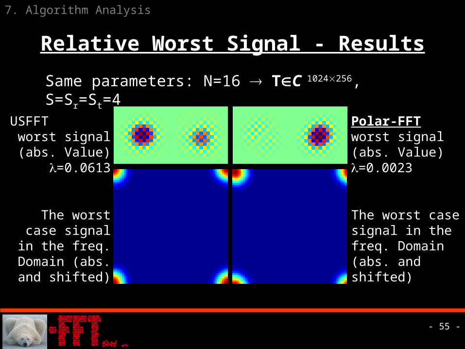
7. Algorithm Analysis
Relative Worst Signal - Results
Same parameters: N=16 TC 1024256, S=Sr=St=4
USFFT worst signal (abs. Value)
=0.0613
The worst case signal in the
freq. Domain (abs. and
shifted)
Polar-FFT worst signal (abs. Value) =0.0023
The worst case signal in the freq. Domain (abs. and shifted)

- 56 -
7. Algorithm Analysis
Comparing Approximations
PolarFFTPolarPolarFFTPolar
H TATA
Solve for the eigenvalue/vectors of the matrix
and obtained ( in ascending order).
Compare to by computing
using the above eigenvectors and compare to .
USFFTA
2N
1kkk x,
k
22kk xPolarUSFFT TA
k

- 57 -
7. Algorithm Analysis
Comparing Approximations - Results
0 200 400 600 800 1000 120010
-10
10-8
10-6
10-4
10-2
100
102
USFFT
Polar-FFT Eigen-
space of the Polar-FFT
Mean Squared Error
[N=32]

- 58 -
Agenda
1. Thinking Polar – Continuum
2. Thinking Polar – Discrete
3. Current State-Of-The-Art
4. Our Approach - General
5. The Pseudo-Polar Fast Transform
6. From Pseudo-Polar to Polar
7. Algorithm Analysis
8. Conclusions

- 59 -
8. Conclusions
We have proposed a fast, accurate, stable,
and reliable Polar Discrete-Fourier-Transform.
By this we extend utility of FFT algorithms to
new class of settings in image processing.
Future plans: Extend the analysis and improve further,
Demonstrate applications,
Publish the code for the procedure and some applications
over the internet.

- 60 -
Beyond this slides are the appendix
or redundant slides
- 61 -
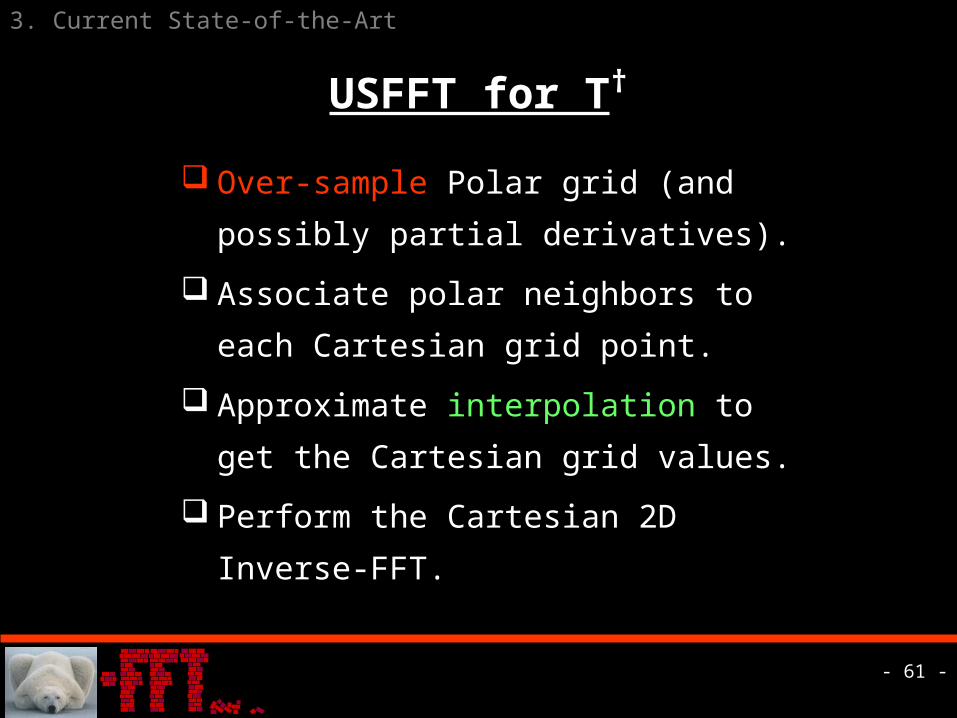
USFFT for T†
3. Current State-of-the-Art
Over-sample Polar grid (and
possibly partial derivatives).
Associate polar neighbors to each
Cartesian grid point.
Approximate interpolation to get
the Cartesian grid values.
Perform the Cartesian 2D Inverse-
FFT.

- 62 -
Our Reading of Literature
3. Current State-of-the-Art
Natterer (1985).
Jackson, Meyer, Nishimura and Macovski (1991).
Schomberg and Timmer (1995).
Choi and Munson (1998).
Direct Fourier method with over-sampling
and interpolation (also called gridding) – see

- 63 -
The Pseudo-Polar Sampling
Basically vertical lines:
12NS
2NSr
y
r
rNS2
12NS
2NSm
yt
x
t
tNSm2
-3 -2 -1 0 1 2 3
-3
-2
-1
0
1
2
3
For St=Sr=1, we have N2 grid points x
y
A. The Fractional Fourier Transform
- 64 -
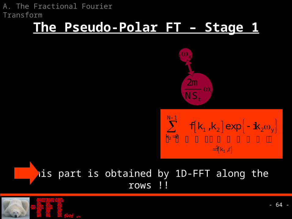
The Pseudo-Polar FT – Stage 1
A. The Fractional Fourier Transform
1 2
1
N 1 N 1
1 y 1 2 2 yk 0 k 0t
f̂ k ,
2mexp ik f k ,k exp ik
NS
This part is obtained by 1D-FFT along the rows !!
1 2
N 1 N 1
x y 1 2 1 x 2 yk 0 k 0
F , f k ,k exp ik ik
1 2
N 1 N 1
1 2 1 y 2 yk 0 k 0 t
2mf k ,k exp ik ik
NS

- 65 -
The Pseudo-Polar FT – Stage 2
1N
0k t
y11yx
1NS
2mikexp,kf̂],m[F,F
The destination grid points are also 1D equi-
spaced in the frequency domain, BUT THEY ARE
NOT IN THE RANGE [-,], but rather [-y,y].
,kf̂ 1 This summation takes columns of (being
equi-spaced 1D signals) and computes Fourier
transform of it.
This task is called Fractional Fourier/Chirp-Z
Transform.
A. The Fractional Fourier Transform

- 66 -
Fractional Fourier Transform
1N
0k Nkm2
iexpkf]m[F
For =1 we get the ordinary 1D-FFT,
For =-1 we get the ordinary 1D-IFFT,
There exists a Fast Fractional Fourier Transform
with the complexity of O(20·Nlog2N), based on 1D-
FFT operations.
See: Fast fractional Fourier transforms and applications, by D. H. Bailey and
P. N. Swarztrauber, SIAM Review, 1991, and also Bluestein, Rabiner, and
Rader (1960’s).
A. The Fractional Fourier Transform

- 67 -
Post Multiplicatio
nConvolution
Pre-Multiplication
1N
0k
2Nk
iNm
i
1N
0k
222
1N
0k
Nmk
iexpekfe
Nmkmk
iexpkf
Nkm2
iexpkf]m[F
22
FR-FFT Detailed
A. The Fractional Fourier Transform
[Back]

- 68 -
Interpolation As 1D Operation
B. From Pseudo-Polar to Polar
1 2
N 1 N 1
1 y 1 2 2 yk 0 k 0t
mexp ik tan f k ,k exp ik
2NS
It is a 1D operation – But it is not the Fractional-FFT.
Can be computed by over-sampled FRFFT and interpolation.
1 2
N 1 N 1
x y 1 2 1 x 2 yk 0 k 0
F , f k ,k exp ik ik
1
N 1
1 y 1k 0 t
m ˆexp ik tan f k ,2NS