( 02/03/2012 )

LLIIDDAARR RREEMMOOTTEE SSEENNSSIINNGG DDAATTAA CCOOLLLLEECCTTIIOONN:: CCAAMMAASS NNAATTIIOONNAALL WWIILLDDLLIIFFEE RREEFFUUGGEE,, IIDDAAHHOO

TABLE OF CONTENTS

1. Overview ......................................................................................... 4

2. Acquisition ....................................................................................... 5

2.1 Airborne Survey – Instrumentation and Methods ....................................... 5

2.2 Ground Survey – Instrumentation and Methods ........................................ 6

2.2.1 Instrumentation ....................................................................... 6

2.2.2 Methodology ............................................................................ 7

3. LiDAR Data Processing ......................................................................... 9

3.1 Applications and Work Flow Overview .................................................. 9

3.2 Aircraft Kinematic GPS and IMU Data ................................................... 9

3.3 Laser Point Processing ................................................................... 10

3.4 Contour Development .................................................................... 12

4. LiDAR Accuracy Assessment ................................................................. 13

4.1 Laser Noise and Relative Accuracy ..................................................... 13

4.2 Absolute Accuracy ........................................................................ 13

5. Study Area Results ............................................................................ 14

5.1 Data Summary: Camas National Wildlife Refuge ..................................... 14

5.1.1 Data Density/Resolution............................................................ 15

5.1.2 Relative Accuracy Calibration Results ............................................ 18

5.1.3 Absolute Accuracy ................................................................... 19

5.1.4 Accuracy per Land Cover ........................................................... 20

6. Model Development ......................................................................... 21

6.1 Hydro Flattened & Breakline Enforced Terrain Models ............................. 21

7. Projection/Datum and Units ................................................................ 23

8. Deliverables ................................................................................... 23

9. Selected Images .............................................................................. 24

10. Glossary ....................................................................................... 27

11. Citations ...................................................................................... 28

Appendix A ........................................................................................ 29

Appendix B ........................................................................................ 30

LiDAR Data Acquisition and Processing: Camas National Wildlife Refuge 2011 Prepared by Watershed Sciences, Inc.

~4~

1. Overview

Watershed Sciences, Inc. (WS) collected Light Detection and Ranging (LiDAR) data for the Camas National Wildlife Refuge in Jefferson County, Idaho from October 19th through the 20th, 2011. This report documents the data acquisition, processing methods, accuracy assessment, and deliverables for this area. The requested area was expanded to include a 100m buffer to ensure complete coverage and adequate point densities around the survey area boundary resulting in a total of 50,015 acres delivered on February 3rd, 2012. Figure 1. Camas National Wildlife Refuge in Jefferson & Clark Counties, Idaho.


~5~

2. Acquisition

2.1 Airborne Survey – Instrumentation and Methods

The 2011 LiDAR survey utilized a mounted Leica ALS50-II sensor in a Cessna Caravan 208B. The ALS50-II sensor operates with Automatic Gain Control (AGC) for intensity correction. The Leica systems were set to acquire 150,000 laser pulses per second (i.e., 150.0 K pulse rate) and flown at 1500 meters above ground level (AGL), capturing a scan angle of ±9o from nadir. With these flight parameters, the laser swath width is ~475 m and the laser pulse footprint is ~34 cm. These settings were developed to yield points with an average native pulse density

of 10 pulses per square meter over terrestrial surfaces. It is not uncommon for some types of surfaces (e.g. dense vegetation or water) to return fewer pulses than the laser originally emitted. These discrepancies between „native‟ and „delivered‟ density will vary depending on terrain, land cover, and the prevalence of water bodies.

The Cessna Caravan is a stable platform, ideal for flying slow and low for high density projects. A Leica ALS50-II sensor head installed in the Caravan is shown on the left.

All areas were surveyed with an opposing flight line side-lap of ≥60% (≥100% overlap) to reduce laser shadowing and increase surface laser painting. The Leica laser systems allow up to four range measurements (returns) per pulse, and all discernable laser returns were processed for the output dataset. To accurately solve for laser point position (geographic coordinates x, y, z), the positional coordinates of the airborne sensor and the attitude of the aircraft were recorded continuously throughout the LiDAR data collection mission. Aircraft position was measured twice per second (2 Hz) by an onboard differential GPS unit. Aircraft attitude was measured 200 times per second (200 Hz) as pitch, roll and yaw (heading) from an onboard inertial measurement unit (IMU). To allow for post-processing correction and calibration, aircraft/sensor position and attitude data are indexed by GPS time.


~6~

2.2 Ground Survey – Instrumentation and Methods

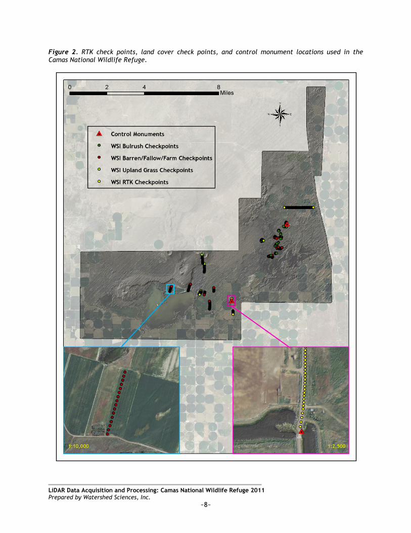
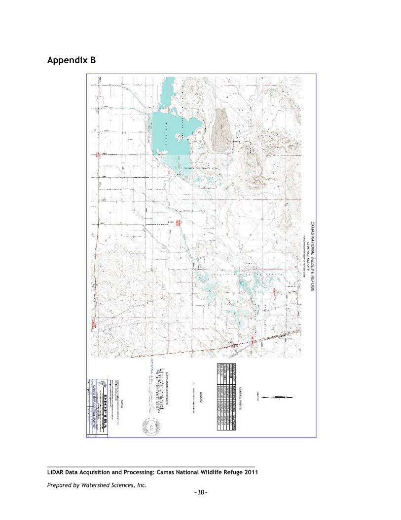
Watershed Sciences coordinated with the U.S. Fish & Wildlife Service (USFWS) to incorporate monuments already identified by Justin M. Steffler of Dioptera (ID PLS 14222) under subcontract with the USFWS. A set of five such monuments were provided to WSI (Appendix B), of which two were used for the Camas survey control. Certification of survey control coordinates by Idaho PLS also provided in Appendix B. During the LiDAR acquisition, static (1 Hz recording frequency) ground surveys were conducted over set monuments. Final monument coordinates used are provided in Table 1 and shown in Figure 2. After the airborne survey, the static GPS data were processed using triangulation with Continuously Operating Reference Stations (CORS) and checked using the Online Positioning User Service (OPUS1) to quantify daily variance. Multiple sessions were processed over the same monument to confirm antenna height measurements and reported position accuracy. Indexed by time, these GPS data were used to correct the continuous onboard measurements of aircraft position recorded throughout the mission. Control monuments were located within 13 nautical miles of the survey area. 2.2.1 Instrumentation

For this project, a Trimble GPS receiver model R7 with Zephyr Geodetic antenna with ground plane was deployed for all static control. A Trimble model R8 GNSS unit was used for collecting check points using real time kinematic (RTK) survey techniques. For RTK data, the collector began recording after remaining stationary for 5 seconds then calculating the pseudo range position from at least three epochs with the relative error under 1.5cm horizontal and 2cm vertical. All GPS measurements were made with dual frequency L1-L2 receivers with carrier-phase correction.

Table 1. Base Station control coordinates for the Camas National Wildlife Refuge remote sensing project.

Base Station ID Datum: NAD83 (CORS96) GRS80

Latitude Longitude Ellipsoid Z (meters)

REFUGE 43 57 08.26.94 N 112 15 29.26934 W 26.296537.34969 W

1452.193

1 Online Positioning User Service (OPUS) is run by the National Geodetic Survey to process corrected monument positions.


~7~

CANAL 43 53 33.06190 N 112 19 03.52151 W 1448.619 2.2.2 Methodology

Each aircraft is assigned a ground crew member with two Trimble R7 receivers and an R8 receiver. The ground crew vehicles are equipped with standard field survey supplies and equipment including safety materials. All control monuments are observed for a minimum of two survey sessions. One of the sessions lasting no fewer than four hours, and the second lasting no fewer than two hours. At the beginning of every session the tripod and antenna are reset, resulting in two independent instrument heights and data files. Data is collected at a rate of 1Hz using a 10 degree mask on the antenna.

The ground crew uploads the GPS data to our FTP site on a daily basis to be returned to the office for review by WSI survey staff, QA/QC review and processing. OPUS processing triangulates the monument position using 3 CORS stations resulting in a fully adjusted position. After multiple days of data have been collected at each monument, accuracy and error ellipses are calculated from the OPUS reports. This information leads to a rating of the monument based on FGDC-STD-007.2-19982 Part 2 table 2.1 at the 95% confidence level. When a statistical stable position is found CORPSCON3 6.0.1 software is used to convert the UTM positions to geodetic positions. This geodetic position is used for processing the LiDAR data.

RTK and aircraft mounted GPS measurements are made during periods with PDOP4 less than or equal to 3.0 and with at least 6 satellites in view of both a stationary reference receiver and the roving receiver. Static GPS data collected in a continuous session average the high PDOP into the final solution in the method used by CORS stations. RTK positions are collected on bare earth locations such as paved, gravel or stable dirt roads, and other locations where the ground is clearly visible (and is likely to remain visible) from the sky during the data acquisition and RTK measurement period(s). RTK positions were also taken in several different habitat types (bulrush, barren\fallow\farm, upland grass, and hard surface) and the results from these vegetation check point sessions are reported in this document.

In order to facilitate comparisons with LiDAR measurements, RTK measurements are not taken on highly reflective surfaces such as center line stripes or lane markings on roads. RTK points were taken no closer than one meter to any nearby terrain breaks such as road edges or drop offs. In addition, USFWS field staff collected check points across land cover types to provide an independent check of the accuracy of the data.

2 Federal Geographic Data Committee Draft Geospatial Positioning Accuracy Standards 3 U.S. Army Corps of Engineers , Engineer Research and Development Center Topographic Engineering Center software 4PDOP: Point Dilution of Precision is a measure of satellite geometry, the smaller the number the better the

geometry between the point and the satellites.


~8~

Figure 2. RTK check points, land cover check points, and control monument locations used in the Camas National Wildlife Refuge.


~9~

3. LiDAR Data Processing

3.1 Applications and Work Flow Overview

1. Resolved kinematic corrections for aircraft position data using kinematic aircraft GPS

and static ground GPS data.

Software: Waypoint GPS v.8.10, Trimble Geomatics Office v.1.62

2. Developed a smoothed best estimate of trajectory (SBET) file that blends post-processed aircraft position with attitude data. Sensor head position and attitude were calculated throughout the survey. The SBET data were used extensively for laser point processing.

Software: IPAS TC v.3.1

3. Calculated laser point position by associating SBET position to each laser point return time, scan angle, intensity, etc. Created raw laser point cloud data for the entire survey in *.las (ASPRS v. 1.2) format.

Software: ALS Post Processing Software v.2.70

4. Imported raw laser points into manageable blocks (less than 500 MB) to perform manual relative accuracy calibration and filter for pits/birds. Ground points were then classified for individual flight lines (to be used for relative accuracy testing and calibration).

Software: TerraScan v.11.007

5. Using ground classified points per each flight line, the relative accuracy was tested. Automated line-to-line calibrations were then performed for system attitude parameters (pitch, roll, heading), mirror flex (scale) and GPS/IMU drift. Calibrations were performed on ground classified points from paired flight lines. Every flight line was used for relative accuracy calibration.

Software: TerraMatch v.11.006

6. Position and attitude data were imported. Resulting data were classified as ground and non-ground points. Statistical absolute accuracy was assessed via direct comparisons of ground classified points to ground RTK survey data. Data were then converted to orthometric elevations (NAVD88) by applying a Geoid03 correction. Software: TerraScan v.11.007, TerraModeler v.11.002

7. Bare Earth models were created as a triangulated surface and exported as ArcInfo ASCII grids and Image files at a 1 meter pixel resolution. Vegetation Canopy Height models (nDSM) were created for any class at 1 meter grid spacing and exported as ArcInfo ASCII grids and Image files.

Software: TerraScan v.11.007, ArcMap v. 9.3.1, TerraModeler v.11.002

3.2 Aircraft Kinematic GPS and IMU Data

LiDAR survey datasets were referenced to the 1 Hz static ground GPS data collected over pre-surveyed monuments with known coordinates. While surveying, the aircraft collected 2 Hz kinematic GPS data, and the onboard inertial measurement unit (IMU) collected 200 Hz aircraft attitude data. Waypoint GPS v.8.10 was used to process the kinematic corrections for the aircraft. The static and kinematic GPS data were then post-processed after the survey to


~10~

obtain an accurate GPS solution and aircraft positions. IPAS TC v.3.1 was used to develop a trajectory file that includes corrected aircraft position and attitude information. The trajectory data for the entire flight survey session were incorporated into a final smoothed best estimated trajectory (SBET) file that contains accurate and continuous aircraft positions and attitudes.

3.3 Laser Point Processing

Laser point coordinates were computed using the IPAS and ALS Post Processor software suites based on independent data from the LiDAR system (pulse time, scan angle), and aircraft trajectory data (SBET). Laser point returns (first through fourth) were assigned an associated (x, y, z) coordinate along with unique intensity values (0-255). The data were output into large LAS v. 1.2 files with each point maintaining the corresponding scan angle, return number (echo), intensity, and x, y, z (easting, northing, and elevation) information. These initial laser point files were too large for subsequent processing. To facilitate laser point processing, bins (polygons) were created to divide the dataset into manageable sizes (< 500 MB). Flightlines and LiDAR data were then reviewed to ensure complete coverage of the survey area and positional accuracy of the laser points. Laser point data were imported into processing bins in TerraScan, and manual calibration was performed to assess the system offsets for pitch, roll, heading and scale (mirror flex). Using a geometric relationship developed by Watershed Sciences, each of these offsets was resolved and corrected if necessary. LiDAR points were then filtered for noise, pits (artificial low points), and birds (true birds as well as erroneously high points) by screening for absolute elevation limits, isolated points and height above ground. Each bin was then manually inspected for remaining pits and birds and spurious points were removed. In a bin containing approximately 7.5-9.0 million points, an average of 50-100 points are typically found to be artificially low or high. Common sources of non-terrestrial returns are clouds, birds, vapor, haze, decks, brush piles, etc. Internal calibration was refined using TerraMatch. Points from overlapping lines were tested for internal consistency and final adjustments were made for system misalignments (i.e., pitch, roll, heading offsets and scale). Automated sensor attitude and scale corrections yielded 3-5 cm improvements in the relative accuracy. Once system misalignments were corrected, vertical GPS drift was then resolved and removed per flight line, yielding a slight improvement (<1 cm) in relative accuracy. The TerraScan software suite is designed specifically for classifying near-ground points (Soininen, 2004). The processing sequence began by „removing‟ all points that were not „near‟ the earth based on geometric constraints used to evaluate multi-return points. The resulting

LiDAR tree point cloud displayed by RGB values from orthophotos Ground penetration decreases below dense

vegetation


~11~

bare earth (ground) model was visually inspected and additional ground point modeling was performed in site-specific areas to improve ground detail. This manual editing of ground often occurs in areas with known ground modeling deficiencies, such as: bedrock outcrops, cliffs, deeply incised stream banks, and dense vegetation. In some cases, automated ground point classification erroneously included known vegetation (i.e., understory, low/dense shrubs, etc.). These points were manually reclassified. Ground surface rasters were then developed from triangulated irregular networks (TINs) of ground points. To develop the highest hit and vegetation models, buildings and structures were classified through automated point processing algorithms and then manually inspected and edited during the ground model inspection. Typically, manual editing of non-vegetation (building, utility, or mobile devices) classification was necessary where dense canopy was immediately proximate to buildings, or where structures such as utility poles or fences mimicked vegetation. The remaining points not classified as ground, default, roads, water, ignored ground, or error points were separated into two vegetation classes; Vegetation consisting of all returns > 0.26 feet from the ground, and vegetation consisting of all returns between the ground and 0.26 feet above the ground. This distinction was necessary because some potential for unclassified ground exists in the dataset. Vegetation classified returns within 0.26 feet of the ground have higher potential to be artifacts of the dataset caused by minor offsets between flightlines (typically < 0.33 feet), isolated noise points, or abrupt discrete terrain features that did not get classified as ground (i.e. small boulders or sharp cliffs). The majority of these points classified (class 5) are valid returns, so the class was retained in the dataset to be incorporated into analyses at the user‟s discretion.

ASPRS Class Definition

1 Default

2 Ground

3 Vegetation (> 0.26 feet)

4 Roads

5 Vegetation (0 - 0.26 feet)

7 Noise/Error Points

9 Water

10 Ignored Ground

Snow level differences between two missions


~12~

3.4 Contour Development

Contour lines were derived at 1 foot intervals from ground-classified LiDAR point data using TerraSolid processing software in MicroStation v. 8.1. Contour generation from LiDAR point data requires a thinning operation in order to reduce contour sinuosity. Parameters for these operations are: thinning elevation bounds: +/- 0.25ft (0.076m); search radius: 20ft (6.09m). The thinning operation reduces point density where topographic change is minimal (flat surfaces) while preserving resolution where topographic change is present. The total sum of potential error in vertical position is equal to twice the point processing limits (0.50ft/0.152m) plus twice the 2-sigma absolute vertical accuracy value for this dataset. Ground point density rasters were created within MicroStation using a 0.25 foot step resolution and a 6 foot sampling radius. Areas with less than 0.25 ground-classified points per square meter were considered “sparse” and areas with higher densities were considered “covered”. The ground point density raster data are in ESRI GRID format and have a 1 foot pixel resolution. The contour lines were intersected with ground point density raster data, allowing the addition of a confidence attribute to contour lines. Contour lines over “sparse” areas have low confidence, while contour lines over “covered” areas have a high confidence. Areas with low ground point density are commonly beneath buildings and bridges, in locations with dense vegetation, over water, and in other areas where laser penetration to the ground surface is impeded. Figure 3 is an example of a ground point density raster and contour lines. Figure 3. Elevation contours over LiDAR ground-classified point density raster (left) and true-color aerial photograph (right). Red indicates low ground point density and blue represents high density.


~13~

4. LiDAR Accuracy Assessment

4.1 Laser Noise and Relative Accuracy

Laser point absolute accuracy is largely a function of laser noise and relative accuracy. To minimize these contributions to absolute error, we first performed a number of noise filtering and calibration procedures prior to evaluating absolute accuracy.

Laser Noise For any given target, laser noise is the breadth of the data cloud per laser return (i.e., last, first, etc.). Lower intensity surfaces (roads, rooftops, still/calm water) experience higher laser noise. The laser noise range for this survey was approximately 0.02 meters. Relative Accuracy Relative accuracy refers to the internal consistency of the data set - the ability to place a laser point in the same location over multiple flight lines, GPS conditions, and aircraft attitudes. Affected by system attitude offsets, scale, and GPS/IMU drift, internal consistency is measured as the divergence between points from different flight lines within an overlapping area. Divergence is most apparent when flight lines are opposing. When the LiDAR system is well calibrated, the line-to-line divergence is low (<10 cm). See Appendix A for further information on sources of error and operational measures that can be taken to improve relative accuracy. Relative Accuracy Calibration Methodology

1. Manual System Calibration: Calibration procedures for each mission require solving geometric relationships that relate measured swath-to-swath deviations to misalignments of system attitude parameters. Corrected scale, pitch, roll and heading offsets were calculated and applied to resolve misalignments. The raw divergence between lines was computed after the manual calibration was completed and reported for each survey area.

2. Automated Attitude Calibration: All data were tested and calibrated using TerraMatch automated sampling routines. Ground points were classified for each individual flight line and used for line-to-line testing. System misalignment offsets (pitch, roll and heading) and scale were solved for each individual mission and applied to respective mission datasets. The data from each mission were then blended when imported together to form the entire area of interest.

3. Automated Z Calibration: Ground points per line were used to calculate the vertical divergence between lines caused by vertical GPS drift. Automated Z calibration was the final step employed for relative accuracy calibration.

4.2 Absolute Accuracy

Laser point absolute accuracy is largely a function of laser noise and relative accuracy. To minimize these contributions to absolute error, a number of noise filtering and calibration procedures were performed prior to evaluating absolute accuracy. The LiDAR quality assurance process uses the data from the real-time kinematic (RTK) ground survey conducted in the AOI. For this delivery, a total of 481 RTK GPS measurements were collected on hard surfaces distributed among multiple flight swaths. Suitable and accessible hard-surfaces limited the number of RTK points able to be collected. To assess absolute accuracy the


~14~

location coordinates of these known RTK ground points were compared to those calculated for the closest ground-classified laser points. The vertical accuracy of the LiDAR data is described as the mean and standard deviation

(sigma ~ ) of divergence of LiDAR point coordinates from RTK ground survey point coordinates. To provide a sense of the model predictive power of the dataset, the root mean square error (RMSE) for vertical accuracy is also provided. These statistics assume the error distributions for x, y, and z are normally distributed, thus the skew and kurtosis of distributions are considered when evaluating error statistics. Statements of statistical accuracy apply to fixed terrestrial surfaces only and may not be applied to areas of dense vegetation or steep terrain (See Appendix A).

5. Study Area Results

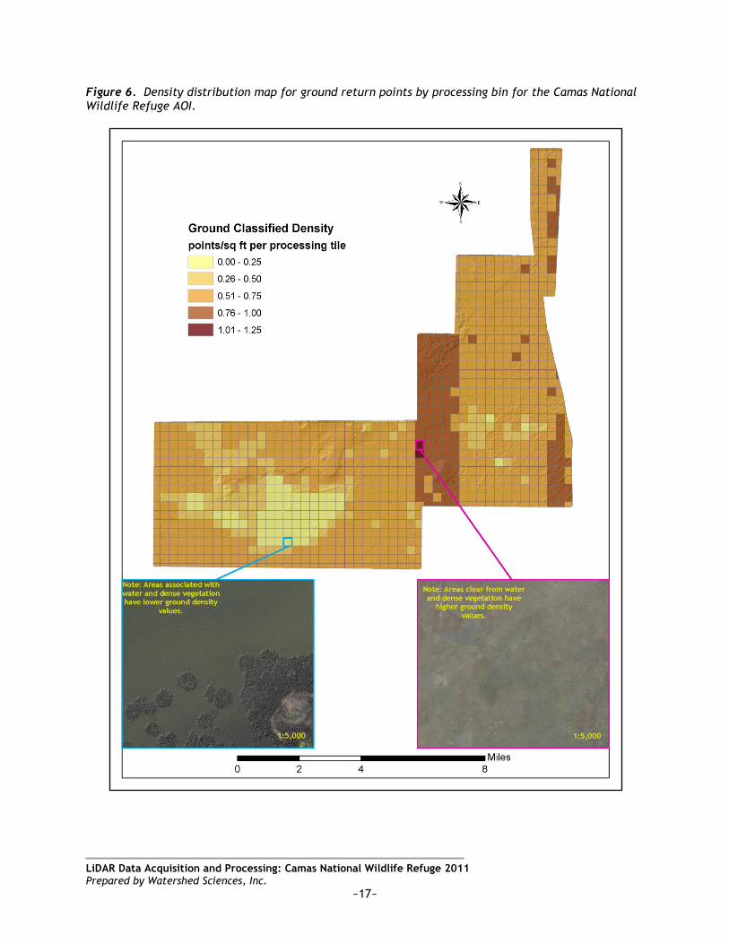
Summary statistics for accuracy (relative and absolute) and point resolution of the LiDAR data collected in Camas National Wildlife Refuge area are presented below in terms of central tendency, variation around the mean, and the spatial distribution of the data (for point resolution by tile). The initial dataset, acquired to be ≥10 points per square meter, was filtered as described previously to remove spurious or inaccurate points. Additionally, some types of surfaces (i.e., dense vegetation, breaks in terrain, water, steep slopes) may return fewer pulses (delivered density) than the laser originally emitted (native density). Ground classifications were derived from automated ground surface modeling and manual, supervised classifications where it was determined that the automated model had failed. Ground return densities will be lower in areas of dense vegetation, water, or buildings. In addition to the hard surface RTK data collection, points were also collected independently on three different land cover types within in the Camas National Wildlife Refuge area by Watershed Sciences. Individual accuracies were calculated for each land-cover type to assess confidence in the LiDAR derived ground models across land-cover classes. The land cover classes for this project include:

Bulrush

Upland Grass

Barren/Fallow/Farm (Cultivated field)

Hard Surface/Bare Earth

5.1 Data Summary: Camas National Wildlife Refuge

Table 2. LiDAR Resolution and Accuracy - Specifications and Achieved Values

Targeted Achieved

Resolution: ≥ 10 points/m2 13.185 points/m2

*Vertical Accuracy ( ): < 0.8 ft (24.5 cm) 0.081 ft (2.46 cm)


~15~

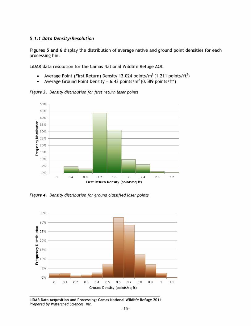
5.1.1 Data Density/Resolution

Figures 5 and 6 display the distribution of average native and ground point densities for each processing bin.

LiDAR data resolution for the Camas National Wildlife Refuge AOI:

Average Point (First Return) Density 13.024 points/m2 (1.211 points/ft2)

Average Ground Point Density = 6.43 points/m2 (0.589 points/ft2)

Figure 3. Density distribution for first return laser points

Figure 4. Density distribution for ground classified laser points


~16~

Figure 5. Density distribution map for first return points by processing bin for the Camas National Wildlife Refuge area.


~17~

Figure 6. Density distribution map for ground return points by processing bin for the Camas National Wildlife Refuge AOI.

LiDAR Data Acquisition and Processing: Camas National Wildlife Refuge 2011

Prepared by Watershed Sciences, Inc.

~18~

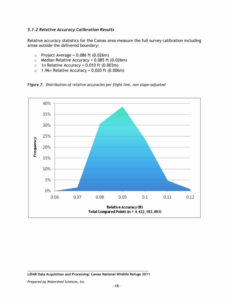
5.1.2 Relative Accuracy Calibration Results

Relative accuracy statistics for the Camas area measure the full survey calibration including areas outside the delivered boundary:

o Project Average = 0.086 ft (0.026m) o Median Relative Accuracy = 0.085 ft (0.026m)

o 1 Relative Accuracy = 0.010 ft (0.003m)

o 1.96 Relative Accuracy = 0.020 ft (0.006m)

Figure 7. Distribution of relative accuracies per flight line, non slope-adjusted



~19~

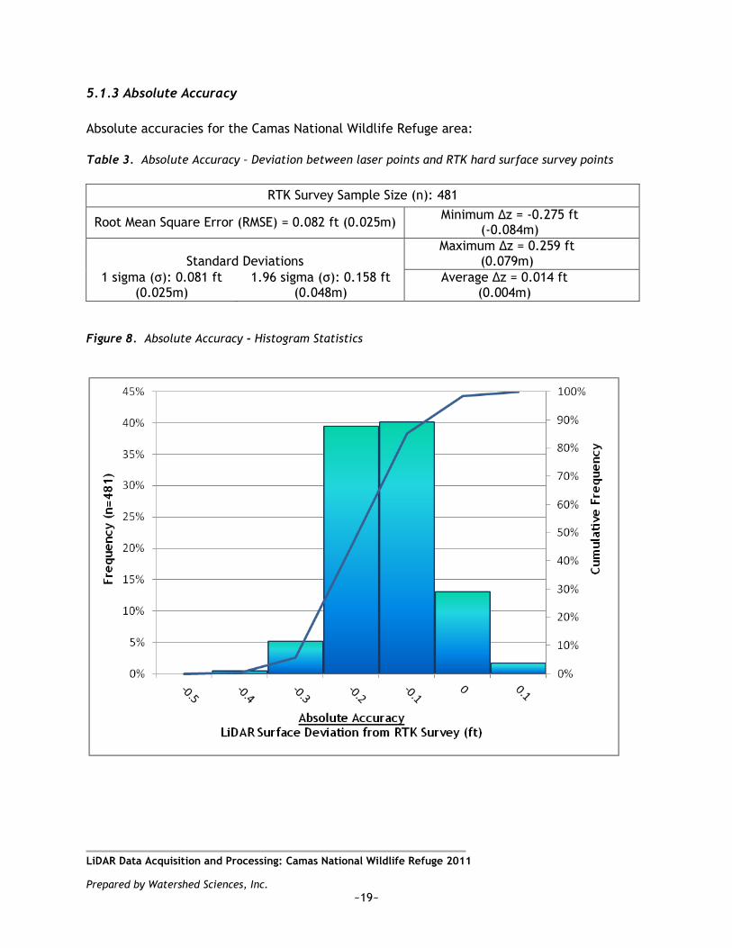
5.1.3 Absolute Accuracy

Absolute accuracies for the Camas National Wildlife Refuge area:

Table 3. Absolute Accuracy – Deviation between laser points and RTK hard surface survey points

RTK Survey Sample Size (n): 481

Root Mean Square Error (RMSE) = 0.082 ft (0.025m) Minimum ∆z = -0.275 ft

(-0.084m)

Standard Deviations Maximum ∆z = 0.259 ft

(0.079m)

1 sigma (σ): 0.081 ft (0.025m)

1.96 sigma (σ): 0.158 ft (0.048m)

Average ∆z = 0.014 ft (0.004m)

Figure 8. Absolute Accuracy - Histogram Statistics



~20~

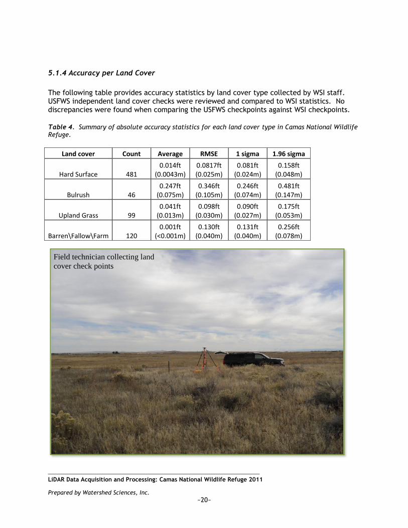
5.1.4 Accuracy per Land Cover

The following table provides accuracy statistics by land cover type collected by WSI staff. USFWS independent land cover checks were reviewed and compared to WSI statistics. No discrepancies were found when comparing the USFWS checkpoints against WSI checkpoints.

Table 4. Summary of absolute accuracy statistics for each land cover type in Camas National Wildlife Refuge.

Land cover Count Average RMSE 1 sigma 1.96 sigma

Hard Surface 481 0.014ft

(0.0043m) 0.0817ft (0.025m)

0.081ft (0.024m)

0.158ft (0.048m)

Bulrush 46 0.247ft

(0.075m) 0.346ft

(0.105m) 0.246ft

(0.074m) 0.481ft

(0.147m)

Upland Grass 99 0.041ft

(0.013m) 0.098ft

(0.030m) 0.090ft

(0.027m) 0.175ft

(0.053m)

Barren\Fallow\Farm 120 0.001ft

(<0.001m) 0.130ft

(0.040m) 0.131ft

(0.040m) 0.256ft

(0.078m)

Field technician collecting land

cover check points



~21~

6. Model Development

6.1 Hydro Flattened & Breakline Enforced Terrain Models

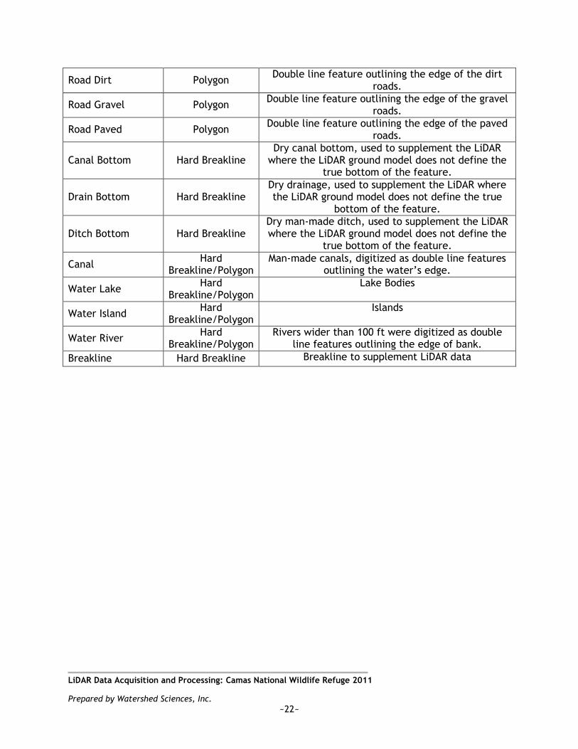
David C. Smith and Associates (DSA), Portland, OR created breaklines and polygons for Camas NWR using LiDAR-grammetry techniques. Table 5 describes the type and definition of each breakline/polygon collected. The breaklines were used to supplement the LiDAR data in creation of a hydro-flattened ground model. A breakline was created around lakes and ponds with areas larger than ~2 acres. Rivers with widths greater than ~100ft were represented as a double line feature and flatten from side-to-side. Road crossings (i.e. culverts and bridges) were removed from the ground model to accurately depict the underlying terrain. The polygons were used to classify the roads and water bodies in the LiDAR.

Water boundaries were enforced using hard breaklines and water surfaces were flattened based on the elevation from the breaklines. The polygons were used to reassign any ground classified points within the water delineated areas to a water class.

Road polygons were used to reassign any ground classified points within the road delineated areas to a road class.

Hard breaklines (lake edges, islands, etc.) were incorporated into the TIN by enforcing triangle edges (adjacent to the breakline) to the elevation values derived from the LiDAR-grammetric breakline. This implementation corrected interpolation along the hard edge.

LiDAR data points within one foot of a breakline (as per USGS specifications) were ignored from the ground classification, giving precedence to breakline Z values.

LiDAR data points within 4.5 feet of a culvert breakline were ignored from the ground classification, in order to give precedence to the underlying terrain.

Table 5. Breaklines/Polygons collected for Camas NWR.

Feature Implementation Description

Culvert Hard Breakline Culverts connecting visible water on each end (high

confidence).

Culvert Connect Hard Breakline Culverts connecting visible water on each or one

end (lower confidence).

Culvert Dry Hard Breakline Culverts connecting dry ditches or drains, digitized

level holding the highest end elevation (high confidence).

Culvert Dry Connect

Hard Breakline Culverts connecting dry ditches or drains, digitized

level holding the highest end elevation (lower confidence).

Culvert Hard Breakline Culverts connecting visible water on each end (high

confidence).

Culvert Connect Hard Breakline Culverts connecting visible water on each or one

end (lower confidence).

Road Driveway Polygon Double line feature outlining the edge of the

driveways.



~22~

Road Dirt Polygon Double line feature outlining the edge of the dirt

roads.

Road Gravel Polygon Double line feature outlining the edge of the gravel

roads.

Road Paved Polygon Double line feature outlining the edge of the paved

roads.

Canal Bottom Hard Breakline Dry canal bottom, used to supplement the LiDAR

where the LiDAR ground model does not define the true bottom of the feature.

Drain Bottom Hard Breakline Dry drainage, used to supplement the LiDAR where the LiDAR ground model does not define the true

bottom of the feature.

Ditch Bottom Hard Breakline Dry man-made ditch, used to supplement the LiDAR where the LiDAR ground model does not define the

true bottom of the feature.

Canal Hard

Breakline/Polygon Man-made canals, digitized as double line features

outlining the water‟s edge.

Water Lake Hard

Breakline/Polygon Lake Bodies

Water Island Hard

Breakline/Polygon Islands

Water River Hard

Breakline/Polygon Rivers wider than 100 ft were digitized as double

line features outlining the edge of bank.

Breakline Hard Breakline Breakline to supplement LiDAR data



~23~

7. Projection/Datum and Units

Projection: Idaho State Plane - East

Datum Vertical: NAVD88 Geoid03

Horizontal: NAD83 (CORS 96)

Units: U.S. Survey Feet

8. Deliverables

Point Data:

RAW Data (1 swath/file) (LAS 1.2 format)

All Returns (unclassified, ground, vegetation, roads, noise, ignored ground, and water classes) (LAS 1.2 format)

Model Keypoints (LAS 1.2 format)

Vector Data:

Tile Index of LiDAR Points (Shapefile)

Raster Index for DEMs (Shapefile)

Deliverable Boundary (TAF)(Shapefile)

Hydrologic Breaklines (ESRI file geodatabase format)

Road Breaklines (ESRI file geodatabase format)

RTK points (Shapefile)

SBETs (AscII TXT format)

1ft Contours (DXF format)

Raster Data:

Elevation Models (1.5ft resolution) • Bare Earth Model (IMG format) • Bare Earth Hydro-flattened/Hydro-enforced Model (IMG format) • Vegetation Canopy Height Model (IMG format)

Intensity Images (GeoTIFF format, 1.5ft resolution)

Data Report: Full report containing introduction, methodology, and

accuracy



~24~

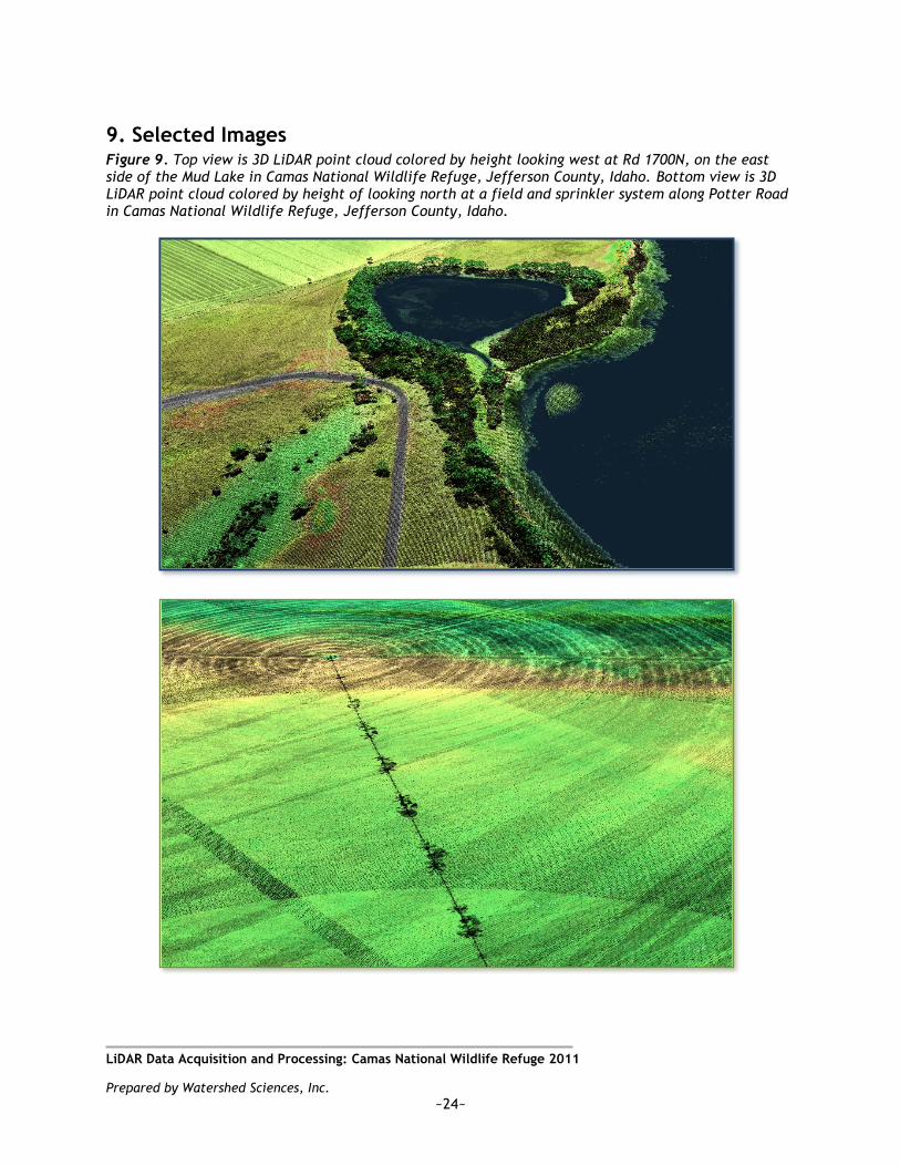
9. Selected Images Figure 9. Top view is 3D LiDAR point cloud colored by height looking west at Rd 1700N, on the east side of the Mud Lake in Camas National Wildlife Refuge, Jefferson County, Idaho. Bottom view is 3D LiDAR point cloud colored by height of looking north at a field and sprinkler system along Potter Road in Camas National Wildlife Refuge, Jefferson County, Idaho.



~25~

Figure 10. Top view is 3D LiDAR point cloud colored by height looking west at an agricultural field along E1800N road and N1100E road in Camas National Wildlife Refuge, Jefferson County, Idaho. Bottom image is 3D LiDAR point cloud colored by height looking west at a farm off of Koefoed Road in the Camas National Wildlife Refuge, in Jefferson County, Idaho.



~26~

Figure 11. Top view is a 3D LiDAR point cloud colored by height looking east at a farm off of Koefoed Road in the Camas National Wildlife Refuge, in Jefferson County, Idaho. The bottom view is also a 3D LiDAR point cloud colored by height looking west at the eastern edge of the Mud Lake in the Camas National Wildlife Refuge, Jefferson County, Idaho.



~27~

10. Glossary 1-sigma (σ) Absolute Deviation: Value for which the data are within one standard deviation

(approximately 68th percentile) of a normally distributed data set.

1.96-sigma (σ) Absolute Deviation: Value for which the data are within two standard deviations

(approximately 95th percentile) of a normally distributed data set.

Root Mean Square Error (RMSE): A statistic used to approximate the difference between real-world points and the LiDAR points. It is calculated by squaring all the values, then taking the average of

the squares and taking the square root of the average.

Pulse Rate (PR): The rate at which laser pulses are emitted from the sensor; typically measured as thousands of pulses per second (kHz).

Pulse Returns: For every laser pulse emitted, the Leica ALS 50 Phase II system can record up to four wave forms reflected back to the sensor. Portions of the wave form that return earliest are the highest element in multi-tiered surfaces such as vegetation. Portions of the wave form that return

last are the lowest element in multi-tiered surfaces.

Accuracy: The statistical comparison between known (surveyed) points and laser points. Typically

measured as the standard deviation (sigma, ) and root mean square error (RMSE).

Intensity Values: The peak power ratio of the laser return to the emitted laser. It is a function of

surface reflectivity.

Data Density: A common measure of LiDAR resolution, measured as points per square meter.

Spot Spacing: Also a measure of LiDAR resolution, measured as the average distance between laser

points.

Nadir: A single point or locus of points on the surface of the earth directly below a sensor as it

progresses along its flight line.

Scan Angle: The angle from nadir to the edge of the scan, measured in degrees. Laser point accuracy

typically decreases as scan angles increase.

Overlap: The area shared between flight lines, typically measured in percents; 100% overlap is

essential to ensure complete coverage and reduce laser shadows.

DTM / DEM: These often-interchanged terms refer to models made from laser points. The digital elevation model (DEM) refers to all surfaces, including bare ground and vegetation, while the digital

terrain model (DTM) refers only to those points classified as ground.

Real-Time Kinematic (RTK) Survey: GPS surveying is conducted with a GPS base station deployed over a known monument with a radio connection to a GPS rover. Both the base station and rover receive differential GPS data and the baseline correction is solved between the two. This type of ground

survey is accurate to 1.5 cm or less.



~28~

11. Citations Soininen, A. 2004. TerraScan User‟s Guide. TerraSolid.



~29~

Appendix A

LiDAR accuracy error sources and solutions:

Type of Error Source Post Processing Solution

GPS (Static/Kinematic)

Long Base Lines None

Poor Satellite Constellation None

Poor Antenna Visibility Reduce Visibility Mask

Relative Accuracy Poor System Calibration

Recalibrate IMU and sensor offsets/settings

Inaccurate System None

Laser Noise

Poor Laser Timing None

Poor Laser Reception None

Poor Laser Power None

Irregular Laser Shape None

Operational measures taken to improve relative accuracy: 1. Low Flight Altitude: Terrain following is employed to maintain a constant above

ground level (AGL). Laser horizontal errors are a function of flight altitude above ground (i.e., ~ 1/3000th AGL flight altitude).

2. Focus Laser Power at narrow beam footprint: A laser return must be received by the system above a power threshold to accurately record a measurement. The strength of the laser return is a function of laser emission power, laser footprint, flight altitude and the reflectivity of the target. While surface reflectivity cannot be controlled, laser power can be increased and low flight altitudes can be maintained.

3. Reduced Scan Angle: Edge-of-scan data can become inaccurate. The scan angle was reduced to a maximum of ±15o from nadir, creating a narrow swath width and greatly reducing laser shadows from trees and buildings.

4. Quality GPS: Flights took place during optimal GPS conditions (e.g., 6 or more satellites and PDOP [Position Dilution of Precision] less than 3.0). Before each flight, the PDOP was determined for the survey day. During all flight times, a dual frequency DGPS base station recording at 1–second epochs was utilized and a maximum baseline length between the aircraft and the control points was less than 19 km (11.5 miles) at all times.

5. Ground Survey: Ground survey point accuracy (i.e. <1.5 cm RMSE) occurs during optimal PDOP ranges and targets a minimal baseline distance of 4 miles between GPS rover and base. Robust statistics are, in part, a function of sample size (n) and distribution. Ground survey RTK points are distributed to the extent possible throughout multiple flight lines and across the survey area.

6. 50% Side-Lap (100% Overlap): Overlapping areas are optimized for relative accuracy testing. Laser shadowing is minimized to help increase target acquisition from multiple scan angles. Ideally, with a 50% side-lap, the most nadir portion of one flight line coincides with the edge (least nadir) portion of overlapping flight lines. A minimum of 50% side-lap with terrain-followed acquisition prevents data gaps.

7. Opposing Flight Lines: All overlapping flight lines are opposing. Pitch, roll and heading errors are amplified by a factor of two relative to the adjacent flight line(s), making misalignments easier to detect and resolve.



~30~

Appendix B

( 02/03/2012 ) - FWS

Documents

Transcript of ( 02/03/2012 ) - FWS